ARMA/ARIMA/SARIMA Models

1 ARIMA Modeling

In this part, I first use the weekly sales of type A stores from the Walmart dataset mentioned in Data Visualization and EDA tab.

1.1 Check the stationarity

This is a visualization of this time series.

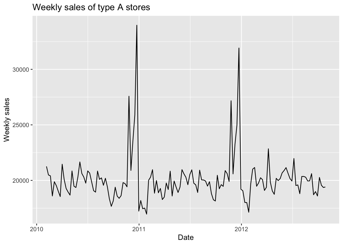
Now review the ACF, PACF and Augmented Dickey-Fuller Test in EDA tab.

Code

ggAcf(temp.ts,150)+ggtitle("ACF graph of the weekly sales")

Code

ggPacf(temp.ts,150)+ggtitle("PACF graph of the weekly sales")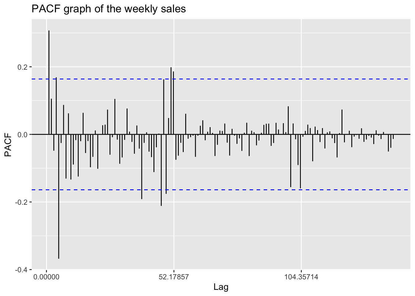

According to the ACF and PACF plots, this time series shows good stationarity besides a extreme value in ACF plot at the lag 52.

Code

adf.test(temp.ts)

    Augmented Dickey-Fuller Test

data:  temp.ts
Dickey-Fuller = -5.3171, Lag order = 5, p-value = 0.01
alternative hypothesis: stationary

As for the ADF test, since p-value is less than 0.05, we have enough evidence to reject the null hypothesis and assert that this time series is stationary.

1.2 Determine the parameter

Now use the ACF and PACF again to determine the parameter p and q in the ARIMA model.

Code

ggAcf(temp.ts,150)+ggtitle("ACF graph of the weekly sales")

From this ACF plot, we can observe that q is likely to be 1, 2, or 5.

Code

ggPacf(temp.ts,150)+ggtitle("PACF graph of the weekly sales")

From this PACF plot, we can predict that p is likely to be 1, 4, or 5. Since we have not differenced the series, d is 0, and this is actually an ARMA model.

1.3 Fit and choose the model

In this part, I will fit the ARIMA model with all possible parameters mentioned above, and use AIC, BIC and AICc as metrics to choose the best model. Here is the result.

Code

i=1
ls=matrix(rep(NA,6*9),nrow=9) 

for (p in c(1,2,5))
{
  for(q in c(1,4,5))
  {
    model<- Arima(temp.ts, order=c(p,0,q),include.drift = TRUE)
    ls[i,]= c(p,0,q,model$aic,model$bic,model$aicc)
    i=i+1
  }
}

temp= as.data.frame(ls)
names(temp)= c("p","d","q","AIC","BIC","AICc")

knitr::kable(temp)

p	d	q	AIC	BIC	AICc
1	0	1	2599.059	2613.873	2599.497
1	0	4	2575.516	2599.219	2576.591
1	0	5	2566.104	2592.770	2567.458
2	0	1	2595.558	2613.335	2596.176
2	0	4	2576.097	2602.763	2577.451
2	0	5	2568.081	2597.710	2569.748
5	0	1	2581.966	2608.631	2583.319
5	0	4	2580.545	2616.099	2582.945
5	0	5	2573.915	2612.432	2576.737

  p d q      AIC     BIC     AICc
3 1 0 5 2566.104 2592.77 2567.458

We can see that the model with parameters (p,d,q)=(1,0,5) has minimum AIC, BIC and AICc. Therefore, I choose this model as the best model.

Here is the summary of the ARIMA(1,0,5) model.

Code

fit <- Arima(temp.ts, order=c(1,0,5),include.drift = TRUE)
summary(fit)

Series: temp.ts 
ARIMA(1,0,5) with drift 

Coefficients:
         ar1      ma1      ma2      ma3     ma4      ma5   intercept   drift
      0.7632  -0.4402  -0.1257  -0.2495  0.3608  -0.5453  19932.3528  2.9485
s.e.  0.0722   0.0896   0.0762   0.0684  0.0858   0.0835    139.7463  1.8740

sigma^2 = 3291926:  log likelihood = -1274.05
AIC=2566.1   AICc=2567.46   BIC=2592.77

Training set error measures:
                    ME     RMSE     MAE        MPE     MAPE     MASE
Training set -12.95413 1762.885 1152.09 -0.6588532 5.480607 1.960847
                     ACF1
Training set -0.005082284

The equation of this ARIMA model:

\[ X_t-0.7632X_{t-1}=\omega_t-0.4402\omega_{t-1}-0.1257\omega_{t-2}-0.2495\omega_{t-3}+0.3608\omega_{t-4}-0.5453\omega_{t-5}+19932.3528 \]

1.4 Model diagnostic

Code

model_output <- capture.output(sarima(temp.ts, 1,0,5))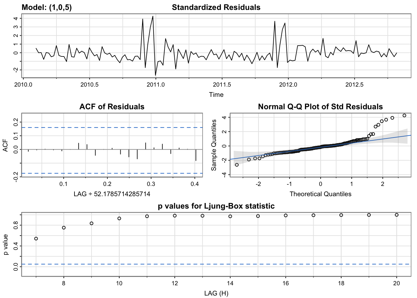

Code

checkresiduals(fit)

    Ljung-Box test

data:  Residuals from ARIMA(1,0,5) with drift
Q* = 6.8906, df = 23, p-value = 0.9995

Model df: 6.   Total lags used: 29

According to the Ljung-Box test, the residuals are independent, which means the model fits this time series well. However, from the Q-Q plot we can observe that a small fraction of the residuals do not follow the normal distribution.

1.5 Auto.arima fitting

Try to use auto.arima function to fit an ARIMA model with this time series:

Code

auto.arima(temp.ts,seasonal = FALSE)

Series: temp.ts 
ARIMA(2,0,2) with non-zero mean 

Coefficients:
          ar1      ar2     ma1     ma2       mean
      -0.9938  -0.3999  1.4020  0.9055  20102.877
s.e.   0.1172   0.1118  0.0735  0.0719    219.415

sigma^2 = 3746572:  log likelihood = -1283.58
AIC=2579.16   AICc=2579.77   BIC=2596.93

Auto.arima chooses parameters (p,d,q)=(2,0,2), which is different from what we have chosen in last part. According to the AIC and BIC, we notice that this model is not so good as the ARIMA(1,0,5) for our time series. The reason auto.arima function makes this choice is perhaps because seasonal component actually exists in the time series and it misleads the auto.arima when this function try to fit an ARIMA model. In fact, a SARIMA model might be better to fit this data than ARIMA model, and I will discuss this later.

1.6 Forecasting

Code

fit %>% forecast(h=12) %>% autoplot()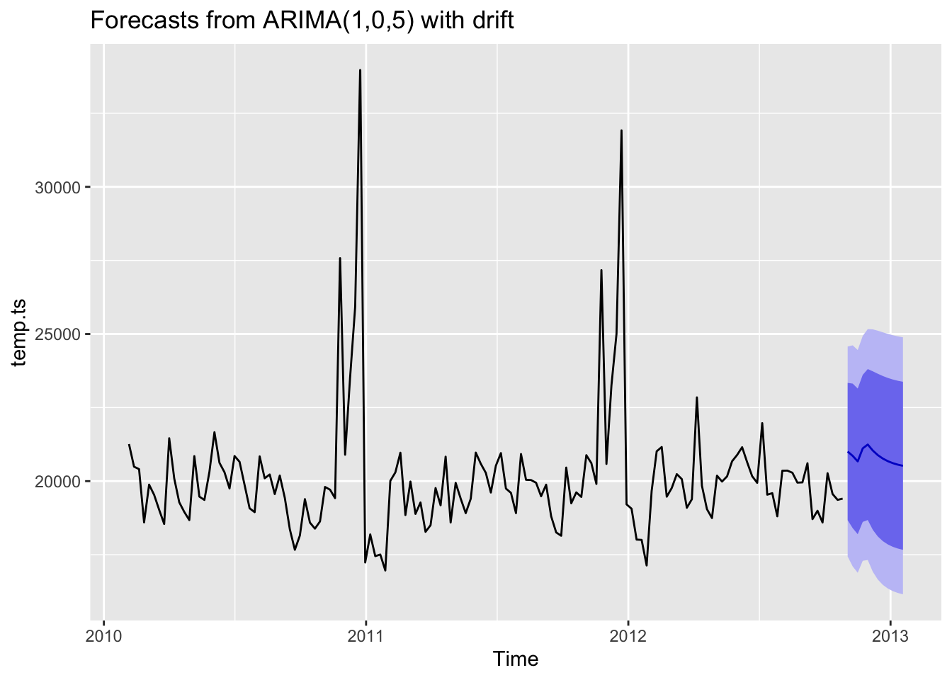

This plot shows the forecasting of next three months and it seems to make sense.

Code

fit %>% forecast(h=52) %>% autoplot()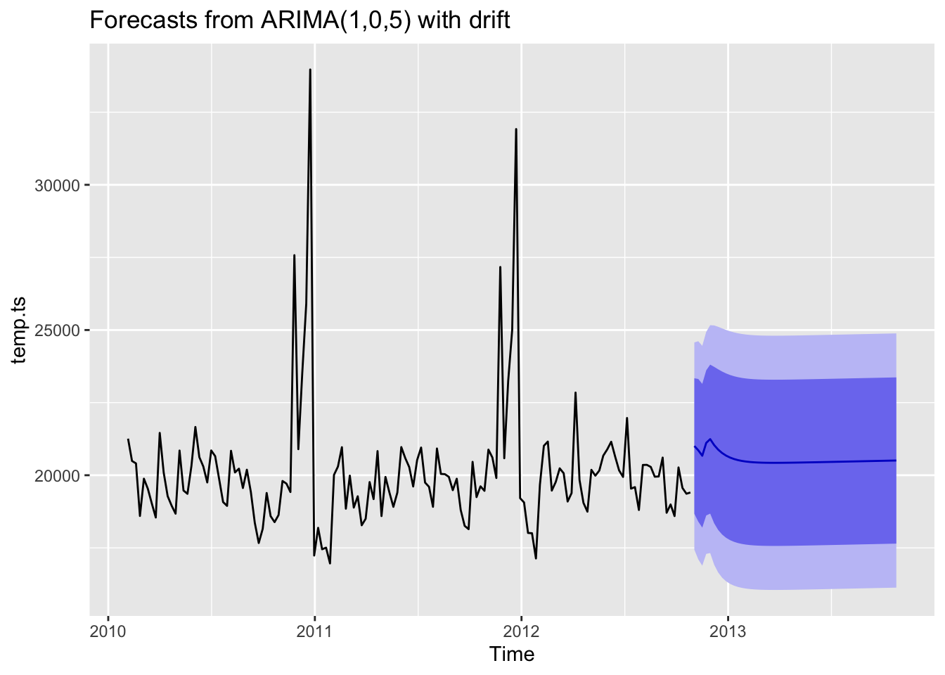

This plot shows the forecasting of next whole year. From this plot, we can clearly see that this ARIMA model actually does not fit the seasonal fluctuations.

1.7 Benchmark comparison

In this part, I will compare the ARIMA model with several benchmark methods, including mean, naive, snaive and drift, using MAE and RMSE.

Use first 120 observations as training data and last 23 observations as test set. Then train the ARIMA model again on the training set.

Code

train = ts(A_sales$avg[1:120], start=decimal_date(as.Date("2010-02-05")), frequency = 365.25/7)
test=temp.ts[121:143]
train_fit=Arima(train, order=c(1,0,5),include.drift = TRUE) 
summary(train_fit)

Series: train 
ARIMA(1,0,5) with drift 

Coefficients:
         ar1      ma1      ma2      ma3     ma4      ma5   intercept   drift
      0.7227  -0.3615  -0.1676  -0.2783  0.4447  -0.6373  19833.9447  4.7891
s.e.  0.0846   0.1024   0.0771   0.0738  0.1058   0.0899    175.1524  2.7894

sigma^2 = 3720135:  log likelihood = -1077.18
AIC=2172.36   AICc=2174   BIC=2197.45

Training set error measures:
                   ME     RMSE      MAE        MPE     MAPE     MASE
Training set 5.740623 1863.364 1262.993 -0.6045651 5.981074 1.939874
                    ACF1
Training set -0.02798821

Code

pred=forecast(train_fit,23)
res=pred$mean-test

pred_mean=meanf(train, h=23)
pred_naive=naive(train, h=23)
pred_snaive=snaive(train, h=23)
pred_drift=rwf(temp.ts, h=23, drift=TRUE)

res_mean=pred_mean$mean-test
res_naive=pred_naive$mean-test
res_snaive=pred_snaive$mean-test
res_drift=pred_drift$mean-test

mae_fit=mean(abs(res))
mae_mean=mean(abs(res_mean))
mae_naive=mean(abs(res_naive))
mae_snaive=mean(abs(res_snaive))
mae_drift=mean(abs(res_drift))

rmse_fit=sqrt(mean(res**2))
rmse_mean=sqrt(mean(res_mean**2))
rmse_naive=sqrt(mean(res_naive**2))
rmse_snaive=sqrt(mean(res_snaive**2))
rmse_drift=sqrt(mean(res_drift**2))

temp=data.frame(
  methods=c("ARIMA", "mean", "naive", "snaive", "drift"),
  MAE=c(mae_fit, mae_mean, mae_naive, mae_snaive, mae_drift),
  RMSE=c(rmse_fit, rmse_mean, rmse_naive, rmse_snaive, rmse_drift)
)
knitr::kable(temp)

methods	MAE	RMSE
ARIMA	778.2579	965.2251
mean	655.3043	819.5058
naive	657.3680	827.9891
snaive	706.8828	952.0468
drift	887.8810	1063.6860

From this result, we can find that the ARIMA model trained on the training set does not perform better than some of the benchmark methods.

Following is a graph that displays the forecasting of ARIMA and benchmark methods for next half year.

Code

autoplot(temp.ts) +
  autolayer(meanf(temp.ts, h=26),
            series="Mean", PI=FALSE) +
  autolayer(naive(temp.ts, h=26),
            series="Naïve", PI=FALSE) +
  autolayer(snaive(temp.ts, h=26),
            series="SNaïve", PI=FALSE)+
  autolayer(rwf(temp.ts, h=26, drift=TRUE),
            series="Drift", PI=FALSE)+
  autolayer(forecast(fit,26), 
            series="fit",PI=FALSE) +
  guides(colour=guide_legend(title="Forecast"))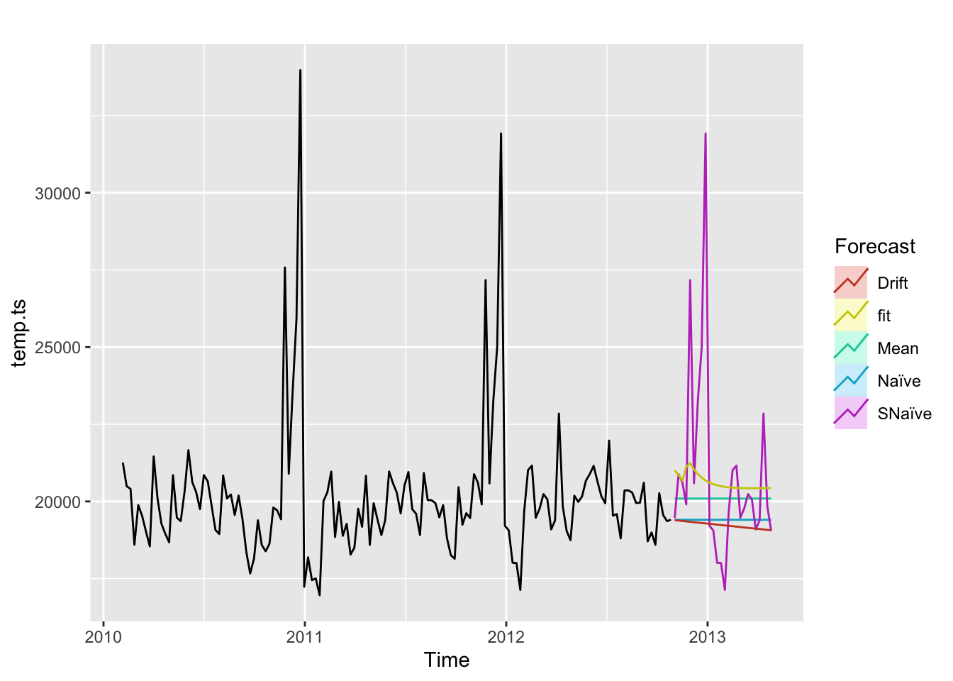

There might be several reasons that this ARIMA model do not perform better than benchmark methods. First, the training set is relatively small, which only contains data almost in two years. Second, there exists seasonal component every year, but a basic ARIMA model can not fit the underline seasonal pattern well. In further analysis, a SARIMA can be used to enhance the performance.

2 SARIMA Modeling

Now, let’s go back to review this ACF plot again.

Code

ggAcf(temp.ts,150)+ggtitle("ACF graph of the weekly sales")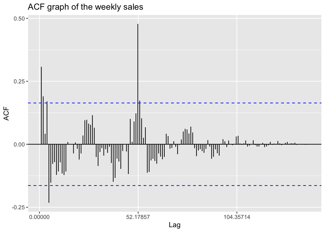

In this plot, it is clear that a significant value appears at lag 52, which is actually the number of weeks in a year. This phenomenon suggests strong seasonal effects in this time series. Therefore, it is appropriate to fit a SARIMA model, which takes seasonal components into consideration, compared to a traditional ARIMA model that we have fitted in the above section.

Additionally, in order to more comprehensively analyze the sales of Walmart, I will also respectively consider the weekly sales of type B and C stores later.

2.1 Differencing and seasonal differencing

Apply first order differencing to the time series and plot:

Code

temp.ts %>% diff() %>% ggtsdisplay()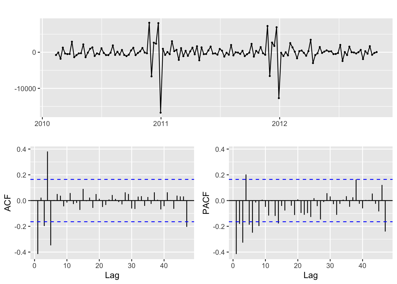

The ACF and PACF show relatively good stationarity.

Now try to apply a seasonal differencing where the seasonal lag is 52.

Code

temp.ts %>% diff(lag=52) %>% ggtsdisplay()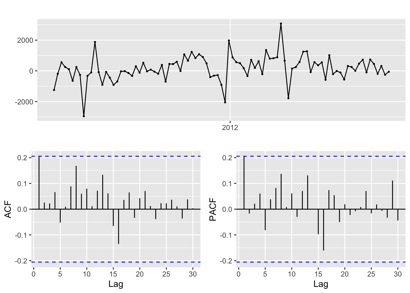

The ACF and PACF indicate much better stationarity compared to first order differencing. Thus, for the parameters of SARIMA model, I will consider:
d=0,1
D=1
p=0,1
P=1,2
q=0,1
Q=1,2

2.2 Fit and choose the model

Code

i=1
ls=matrix(rep(NA,9*12),nrow=12) 

for (p in 0:1)
{
  for(q in 0:1)
  {
    for(P in 1:2)
    {
      for(Q in 1:2)
        {
        for(d in 0:1){
          model<- try(Arima(temp.ts,order=c(p,d,q),seasonal=c(P,1,Q)),silent = TRUE)
          if('try-error' %in% class(model)){
            next
            }else{
            ls[i,]= c(p,d,q,P,1,Q,model$aic,model$bic,model$aicc)
            i=i+1
          }
        }
      }
    }
  }
}

temp= as.data.frame(ls)
names(temp)= c("p","d","q","P","D","Q","AIC","BIC","AICc")

#temp
knitr::kable(temp)

p	d	q	P	D	Q	AIC	BIC	AICc
0	0	0	1	1	1	1480.785	1488.317	1481.061
0	1	0	1	1	1	1506.566	1514.065	1506.845
0	0	0	1	1	2	1482.785	1492.828	1483.250
0	1	0	1	1	2	1508.566	1518.565	1509.036
0	0	1	1	1	1	1480.143	1490.186	1480.608
0	1	1	1	1	1	1463.849	1473.848	1464.320
0	0	1	1	1	2	1482.143	1494.697	1482.849
0	1	1	1	1	2	1465.849	1478.348	1466.563
1	1	0	1	1	1	1491.692	1501.691	1492.163
1	1	0	1	1	2	1493.692	1506.191	1494.406
1	0	1	1	1	1	1482.677	1495.232	1483.383
1	0	1	1	1	2	1484.514	1499.579	1485.514

  p d q P D Q      AIC      BIC    AICc
6 0 1 1 1 1 1 1463.849 1473.848 1464.32

We can see that the model with parameters (p,d,q,P,D,Q)=(0,1,1,1,1,1) has minimum AIC, BIC and AICc. Therefore, I choose this model as the best model.

Here is the summary of the SARIMA(0,1,1,1,1,1,52) model.

Code

fit=Arima(temp.ts,order=c(0,1,1),seasonal=c(1,1,1))
summary(fit)

Series: temp.ts 
ARIMA(0,1,1)(1,1,1)[52] 

Coefficients:
          ma1      sar1      sma1
      -0.9291   -0.3302   -0.0861
s.e.   0.0434  118.5891  141.9681

sigma^2 = 566412:  log likelihood = -727.92
AIC=1463.85   AICc=1464.32   BIC=1473.85

Training set error measures:
                   ME     RMSE      MAE       MPE     MAPE      MASE      ACF1
Training set 68.27586 587.0266 335.8448 0.3596146 1.642288 0.5716048 0.0539026

Model diagnostic:

Code

checkresiduals(fit)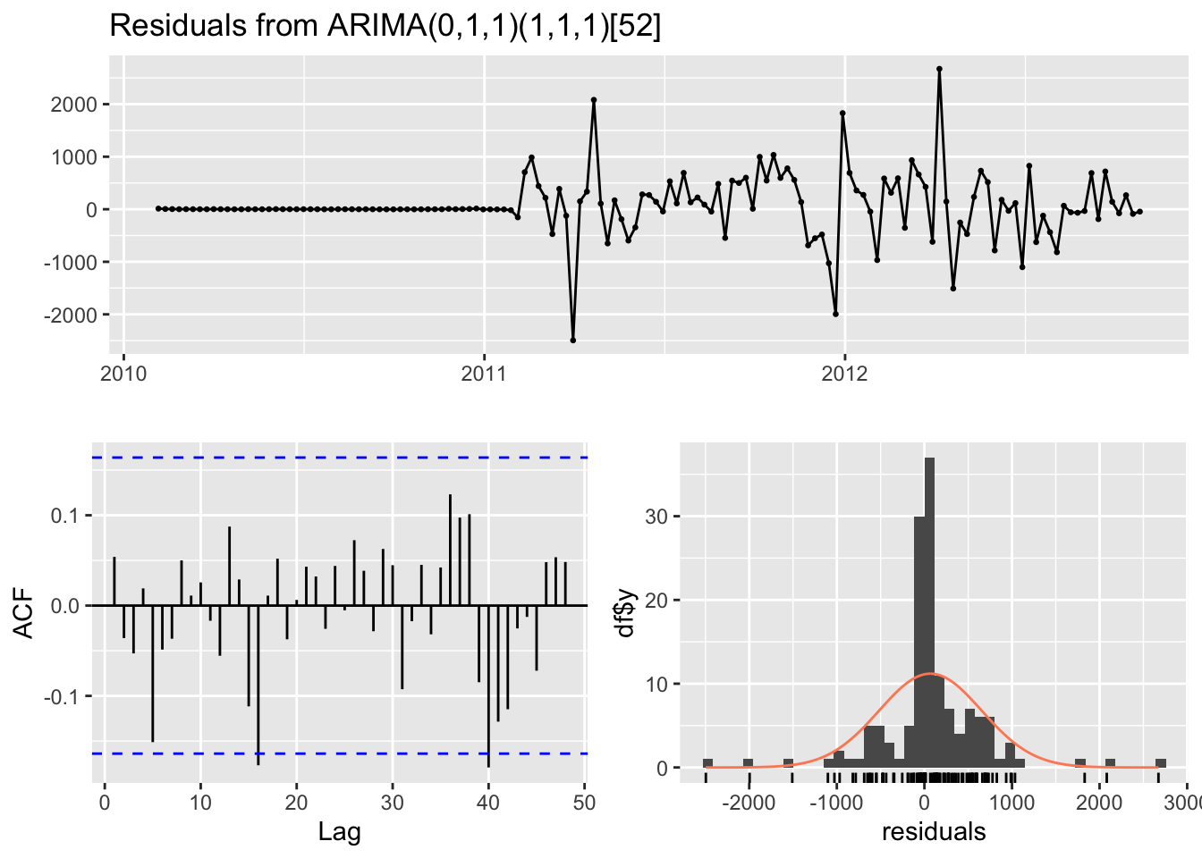

    Ljung-Box test

data:  Residuals from ARIMA(0,1,1)(1,1,1)[52]
Q* = 18.305, df = 26, p-value = 0.8644

Model df: 3.   Total lags used: 29

According to the Ljung-Box test, the residuals are independent, which means the SARIMA model fits this time series well.

2.3 Auto.arima fitting

Try to use auto.arima function to fit a SARIMA model with this time series:

Code

auto.arima(temp.ts,seasonal = TRUE)

Series: temp.ts 
ARIMA(0,1,2)(0,1,0)[52] 

Coefficients:
          ma1      ma2
      -0.7677  -0.1576
s.e.   0.1062   0.1043

sigma^2 = 647091:  log likelihood = -729.61
AIC=1465.21   AICc=1465.49   BIC=1472.71

auto.arima function fits a SARIMA(0,1,2,0,1,0)[52] model, which is different from the SARIMA(0,1,1,1,1,1)[52] that we chose just now. The AIC and AICc of this model is larger than our chosen model, while BIC of this model is slightly smaller due to less parameters. Actually, both models have relatively good performance and they have very close AIC, BIC and AICc values. The results of auto.arima this time make much more sense than in ARIMA section early in this page.

2.4 Forecasting

Code

fit %>% forecast(h=52) %>% autoplot()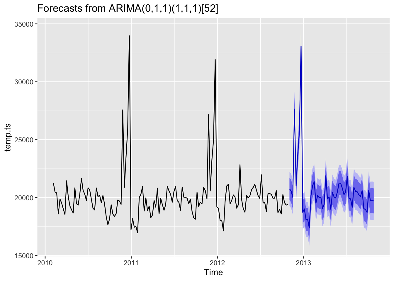

This is the forecasting for the next whole year with our SARIMA model. It is obvious that this model has fitted the seasonal effect quite well.

2.5 Benchmark comparison

Similar to ARIMA section, I will compare the SARIMA model with several benchmark methods, including mean, naive, snaive and drift, using MAE and RMSE.

Use first 120 observations as training data and last 23 observations as test set. Then train the SARIMA model again on the training set.

Code

train = ts(A_sales$avg[1:120], start=decimal_date(as.Date("2010-02-05")), frequency = 365.25/7)
test=temp.ts[121:143]
train_fit=Arima(train,order=c(0,1,1),seasonal=c(1,1,1))
summary(train_fit)

Series: train 
ARIMA(0,1,1)(1,1,1)[52] 

Coefficients:
          ma1     sar1     sma1
      -0.9149  -0.3009  -0.0224
s.e.   0.0512      NaN      NaN

sigma^2 = 724956:  log likelihood = -549.3
AIC=1106.6   AICc=1107.24   BIC=1115.41

Training set error measures:
                   ME     RMSE      MAE      MPE     MAPE      MASE      ACF1
Training set 83.15758 621.8062 338.2122 0.443131 1.647231 0.5194715 0.1017468

Code

pred=forecast(train_fit,23)
res=pred$mean-test

pred_mean=meanf(train, h=23)
pred_naive=naive(train, h=23)
pred_snaive=snaive(train, h=23)
pred_drift=rwf(temp.ts, h=23, drift=TRUE)

res_mean=pred_mean$mean-test
res_naive=pred_naive$mean-test
res_snaive=pred_snaive$mean-test
res_drift=pred_drift$mean-test

mae_fit=mean(abs(res))
mae_mean=mean(abs(res_mean))
mae_naive=mean(abs(res_naive))
mae_snaive=mean(abs(res_snaive))
mae_drift=mean(abs(res_drift))

rmse_fit=sqrt(mean(res**2))
rmse_mean=sqrt(mean(res_mean**2))
rmse_naive=sqrt(mean(res_naive**2))
rmse_snaive=sqrt(mean(res_snaive**2))
rmse_drift=sqrt(mean(res_drift**2))

temp=data.frame(
  methods=c("SARIMA", "mean", "naive", "snaive", "drift"),
  MAE=c(mae_fit, mae_mean, mae_naive, mae_snaive, mae_drift),
  RMSE=c(rmse_fit, rmse_mean, rmse_naive, rmse_snaive, rmse_drift)
)
knitr::kable(temp)

methods	MAE	RMSE
SARIMA	386.7546	482.1954
mean	655.3043	819.5058
naive	657.3680	827.9891
snaive	706.8828	952.0468
drift	887.8810	1063.6860

According to this result table, SARIMA outperforms all the benchmark methods without any doubt. Both MAE and RMSE of the model are much less than benchmarks. This means the SARIMA model performs well and it can fit the pattern within the data.

Following is a graph that displays the forecasting of ARIMA and benchmark methods for next half year.

Code

autoplot(temp.ts) +
  autolayer(meanf(temp.ts, h=26),
            series="Mean", PI=FALSE) +
  autolayer(naive(temp.ts, h=26),
            series="Naïve", PI=FALSE) +
  autolayer(snaive(temp.ts, h=26),
            series="SNaïve", PI=FALSE)+
  autolayer(rwf(temp.ts, h=26, drift=TRUE),
            series="Drift", PI=FALSE)+
  autolayer(forecast(fit,26), 
            series="fit",PI=FALSE) +
  guides(colour=guide_legend(title="Forecast"))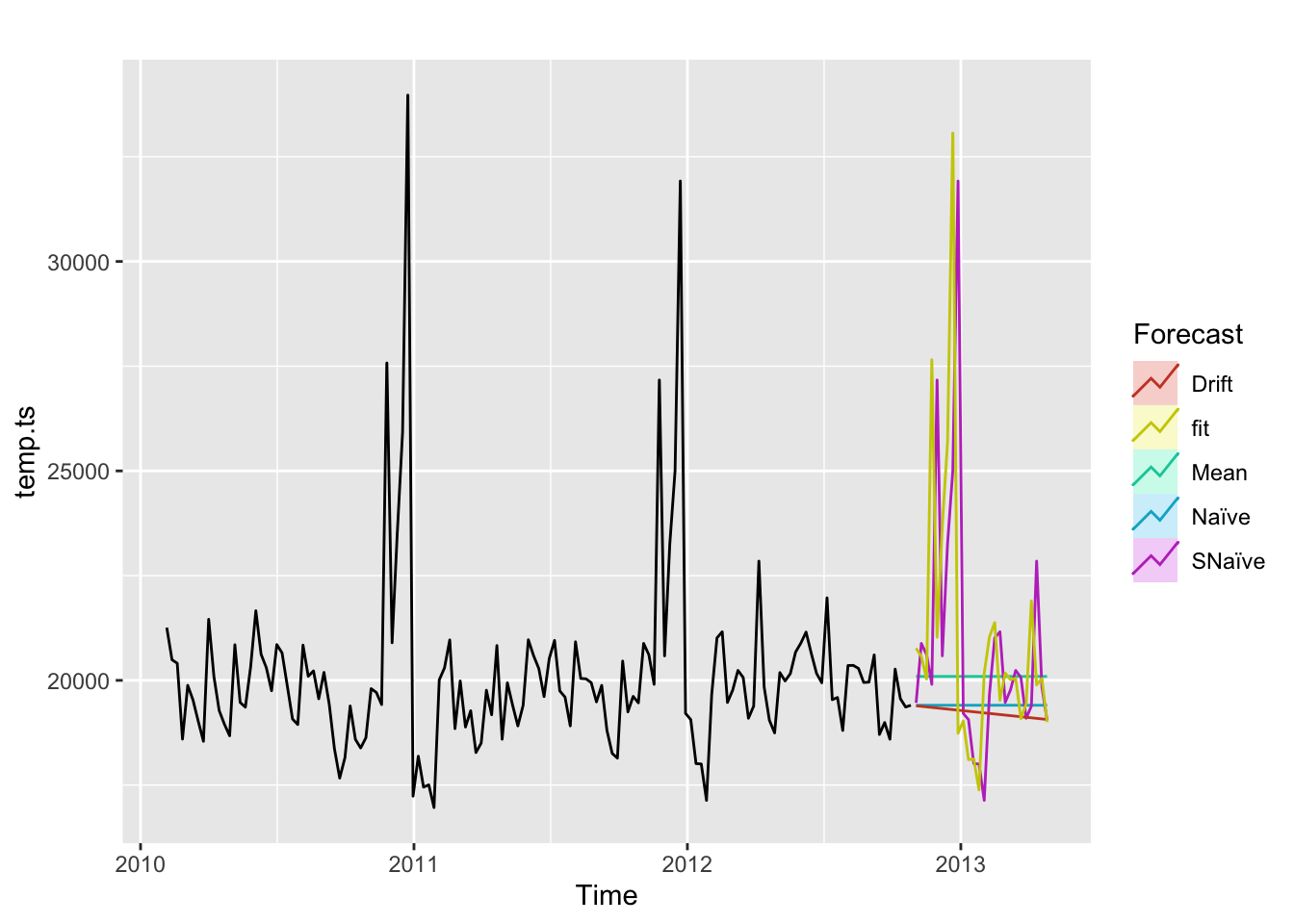

2.6 Cross-validation

In this part, I will try seasonal cross validation using 1 step ahead forecasts and 52 steps (the seasonal period of this data) ahead forecasts and compare the RMSE of our chosen SARIMA model and the auto.arima model.

Code

set.seed(1001)

farima1 <- function(x, h){forecast(Arima(x, order=c(0,1,1),seasonal = c(1,1,1)), h=h)}
farima2 <- function(x, h){forecast(Arima(x, order=c(0,1,2),seasonal = c(0,1,0)), h=h)}

e1 <- tsCV(temp.ts, farima1, h=1)
e2 <- tsCV(temp.ts, farima2, h=1)
RMSE1=sqrt(mean(e1^2, na.rm=TRUE))
RMSE2=sqrt(mean(e2^2, na.rm=TRUE))

e3 <- tsCV(temp.ts, farima1, h=52)
e4 <- tsCV(temp.ts, farima2, h=52)
RMSE3=sqrt(mean(e3^2, na.rm=TRUE))
RMSE4=sqrt(mean(e4^2, na.rm=TRUE))

Code

temp=data.frame(
  Models=c("Chosen model", "Auto model"),
  step_1=c(RMSE1, RMSE2),
  step_52=c(RMSE3, RMSE4)
)
knitr::kable(temp)

Models	step_1	step_52
Chosen model	829.5337	713.0525
Auto model	860.5003	926.7938

This RMSE result table shows that our chosen model SARIMA(0,1,1,1,1,1)[52] have much smaller RMSE for both 1 step and 52 steps cross-validation, which means our model performs better than the model selected by auto.arima.

2.7 Type B and C stores

In this part, I will fit SARIMA models for the weekly sales of type B and C stores. First, let’s have a quick look of these two time series.

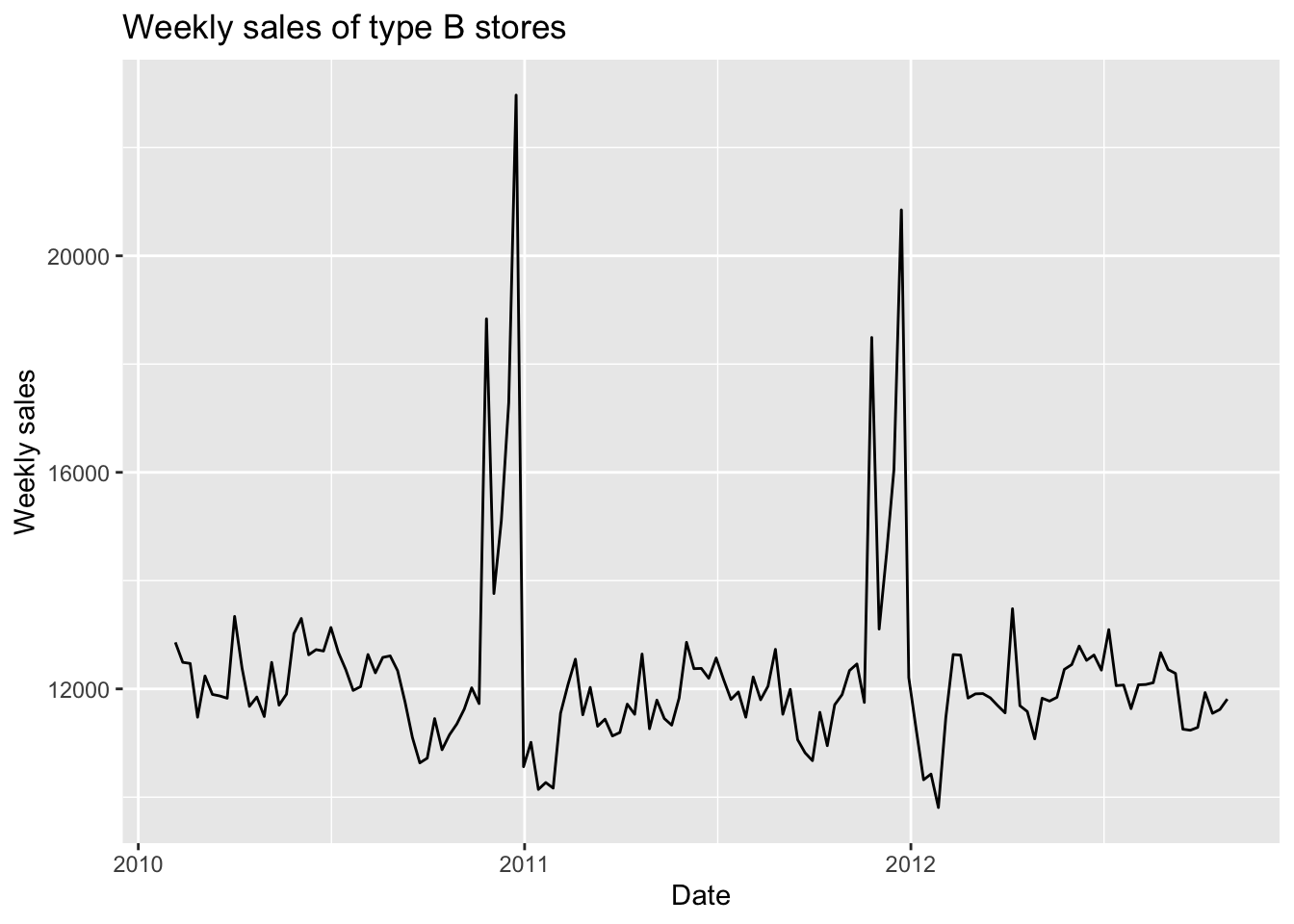
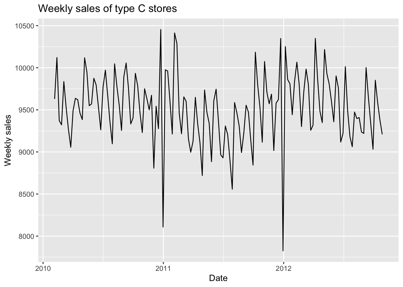
We can notice that the data pattern of type B stores are very similar to type A stores, but the weekly sales of type C stores look quite different.

Now, fit different SARIMA models for type B and C stores then choose the best models based on AIC, BIC and AICc.

Code

i=1
ls=matrix(rep(NA,9*32),nrow=32) 

for (p in 0:1)
{
  for(q in 0:1)
  {
    for(P in 0:1)
    {
      for(Q in 0:1)
        {
        for(d in 0:1){
          model<- try(Arima(temp.ts.b,order=c(p,d,q),seasonal=c(P,1,Q)),silent = TRUE)
          if('try-error' %in% class(model)){
            next
            }else{
            ls[i,]= c(p,d,q,P,1,Q,model$aic,model$bic,model$aicc)
            i=i+1
          }
        }
      }
    }
  }
}

temp= as.data.frame(ls)
names(temp)= c("p","d","q","P","D","Q","AIC","BIC","AICc")

   p d q P D Q      AIC      BIC     AICc
14 0 1 1 1 1 0 1402.548 1410.047 1402.827

For type B stores, the best model with minimum AIC, BIC and AICc is SARIMA(0,1,1,1,1,0)[52]. The parameters of this model is almost the same as those we discussed for type A stores except Q.

Code

fit=Arima(temp.ts.b,order=c(0,1,1),seasonal=c(1,1,0))
fit %>% forecast(h=52) %>% autoplot()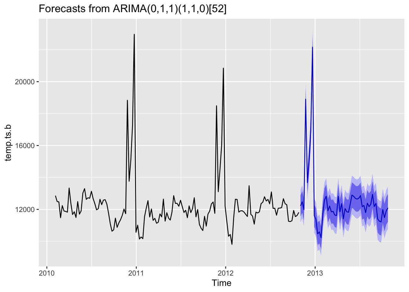

This forecasting above shows that the model captured the seasonal effect well.

Code

i=1
ls=matrix(rep(NA,9*32),nrow=32) 

for (p in 0:1)
{
  for(q in 0:1)
  {
    for(P in 0:1)
    {
      for(Q in 0:1)
        {
        for(d in 0:1){
          model<- try(Arima(temp.ts.c,order=c(p,d,q),seasonal=c(P,1,Q)),silent = TRUE)
          if('try-error' %in% class(model)){
            next
            }else{
            ls[i,]= c(p,d,q,P,1,Q,model$aic,model$bic,model$aicc)
            i=i+1
          }
        }
      }
    }
  }
}

temp= as.data.frame(ls)
names(temp)= c("p","d","q","P","D","Q","AIC","BIC","AICc")

   p d q P D Q      AIC      BIC     AICc
14 0 1 1 1 1 0 1259.452 1266.952 1259.731

As for type C stores, the number of model parameters are exactly the same as type B stores. The optimal model is also SARIMA(0,1,1,1,1,0)[52].

Code

fit=Arima(temp.ts.c,order=c(0,1,1),seasonal=c(1,1,0))
fit %>% forecast(h=52) %>% autoplot()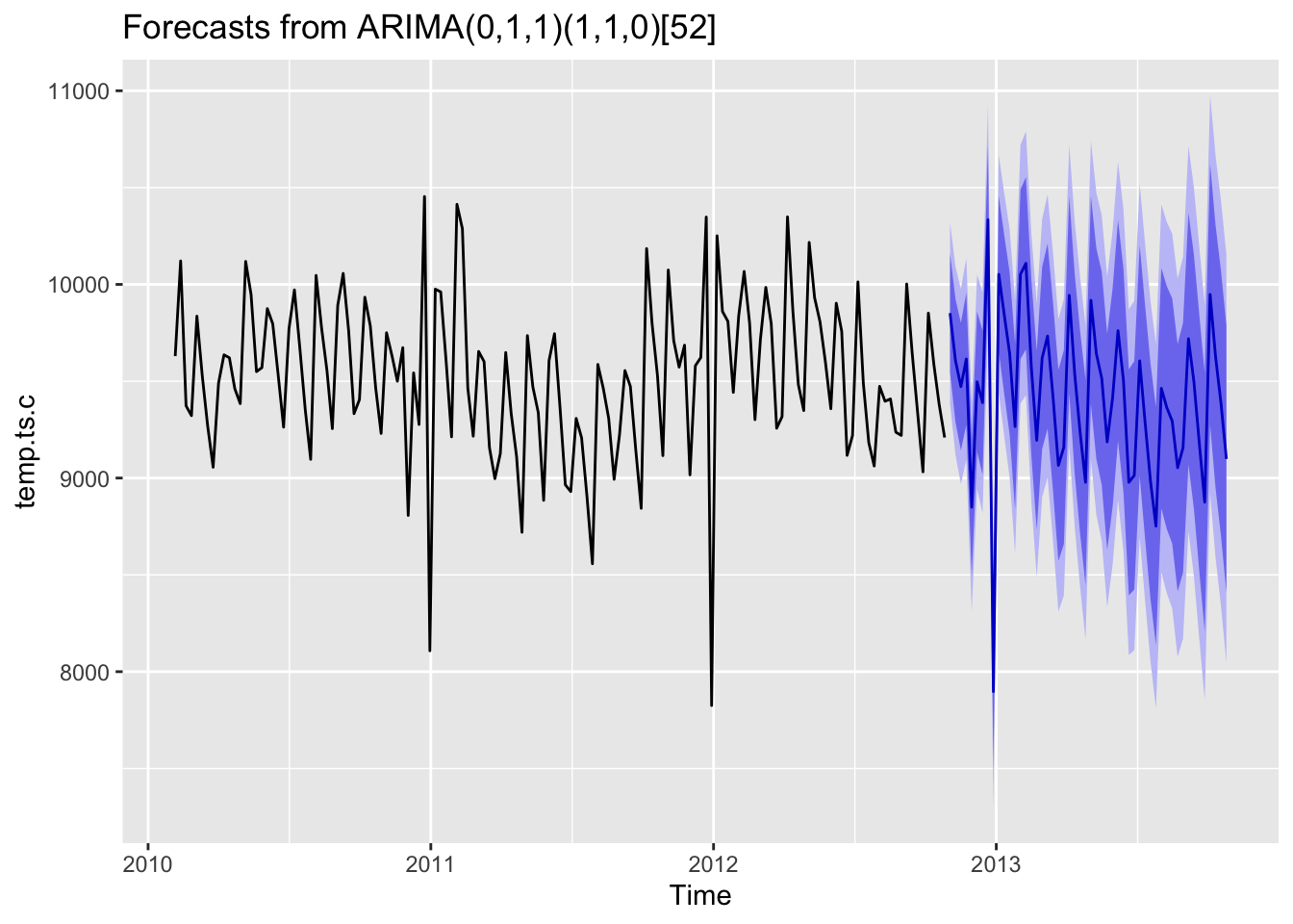

In a conclusion, although type A, B and C stores have different sizes, the SARIMA models fitted with the data have similar parameters and same seasonal period. Additionally, the data patterns of weekly sales for type B and C stores look very different, but the final models of these two types of store selected based on AIC, BIC and AICc have exactly the same numbers of parameters, which suggests that the hidden patterns and seasonal components are actually similar.