Financial Time Series Models (ARCH/GARCH)

Unlike preceding tabs, in this page I will mainly focus on using Autoregressive Conditional Heteroskedasticity model (ARCH), a useful financial time series model, to study the stock price of Walmart since 2010, rather than forecasting the weekly sales as usual. Financial time series data refers to the data collected over time and indicates the changes of financial variables, including stock prices, interest rates, and other financial indicators. A special characteristic of financial time series is that there often exists volatility in the data, and the volatility tends to cluster over time. Under this circumstance, ARCH and GARCH models can be ideal to study the financial time series, since they can take the volatility into consideration.

In this project, I will first train an ARIMA model, and then utilize ARCH or GARCH to fit the residuals of ARIMA model. Thus, the final model for studying this stock price data can be an ARIMA+ARCH/ARIMA+GARCH model.

1 Data gathering and visualization

First, get the stock price data of Walmart from yahoo.

Code

getSymbols("WMT", from="2010-01-01", to="2023-05-02", src="yahoo")

[1] "WMT"

Code

head(WMT)

           WMT.Open WMT.High WMT.Low WMT.Close WMT.Volume WMT.Adjusted
2010-01-04    53.74    54.67   53.67     54.23   20753100     40.01306
2010-01-05    54.09    54.19   53.57     53.69   15648400     39.61462
2010-01-06    53.50    53.83   53.42     53.57   12517200     39.52609
2010-01-07    53.72    53.75   53.26     53.60   10662700     39.54823
2010-01-08    53.43    53.53   53.02     53.33   11363200     39.34901
2010-01-11    53.33    54.44   53.10     54.21   13987700     39.99831

Here is candlestick plot showing the stock price of Walmart since 2010:

Code

chartSeries(WMT, theme = chartTheme("white"),
            bar.type = "hlc",
            up.col = "green", 
            dn.col = "red")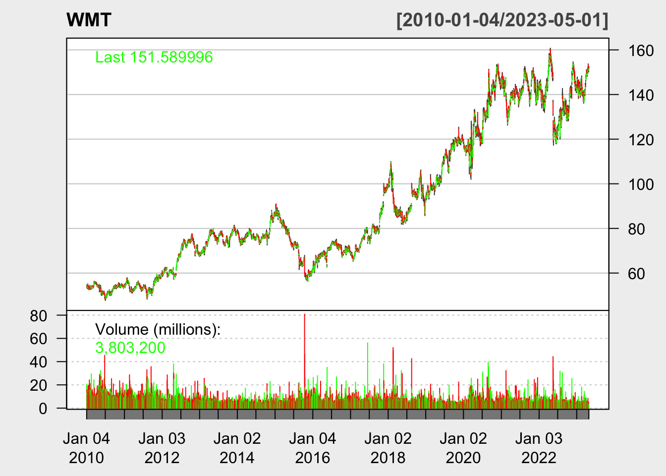

According to this plot, we first notice the upward trend of this stock price within the past decade. Also, this plot shows increasing volatility in the data over time.

Following plot will apply the log function and a first order differencing to the data, which makes it much easier to notice the change in volatility.

Code

WMT.close<- Ad(WMT)

returns = diff(log(WMT.close))

chartSeries(returns, theme="white")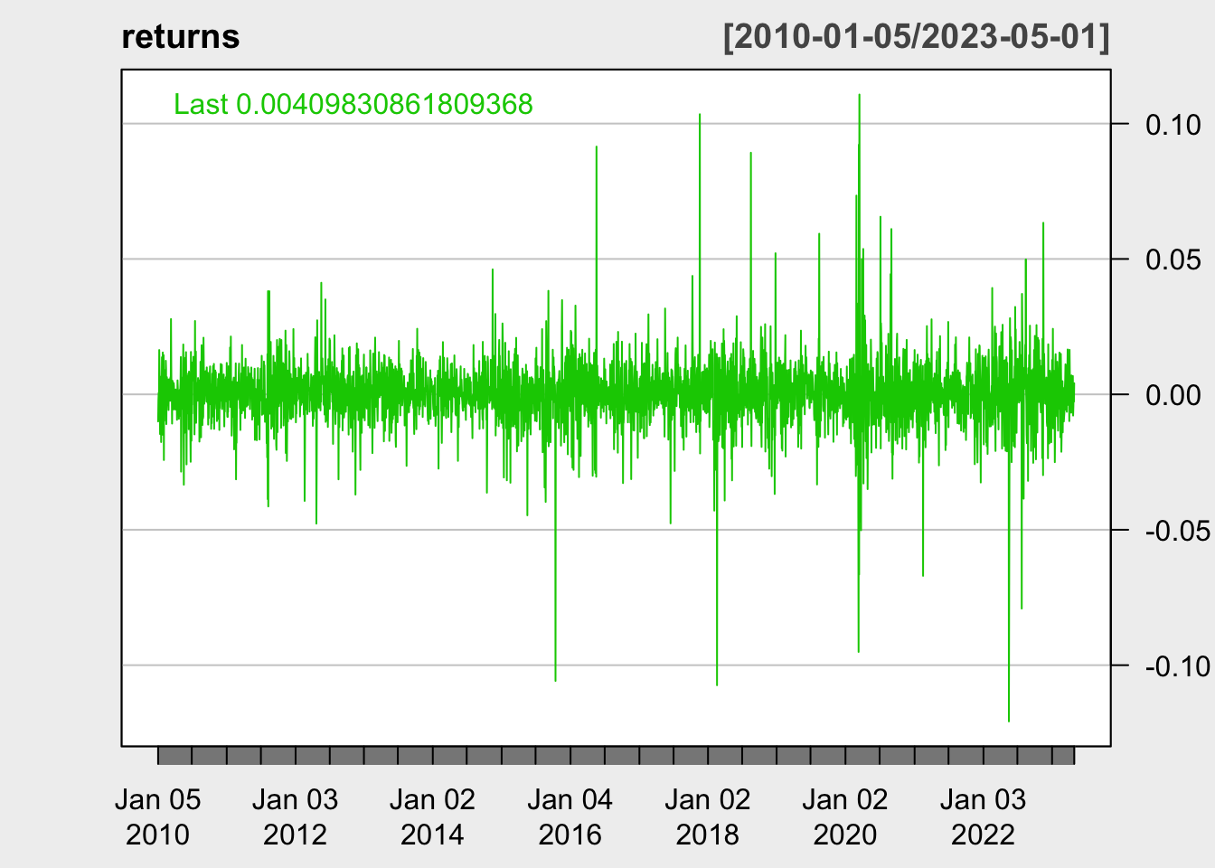

We can clearly see that volatility has greatly increased by years, especially at around 2020. Therefore, an ARCH or GARCH model will be appropriate for studying this data. Now let’s first look at the ACF/PACF plot to check if an ARIMA model is necessary before fitting an ARCH.

2 ACF/PACF plots

Code

ggAcf(log(WMT.close))+ggtitle("ACF plot of log price")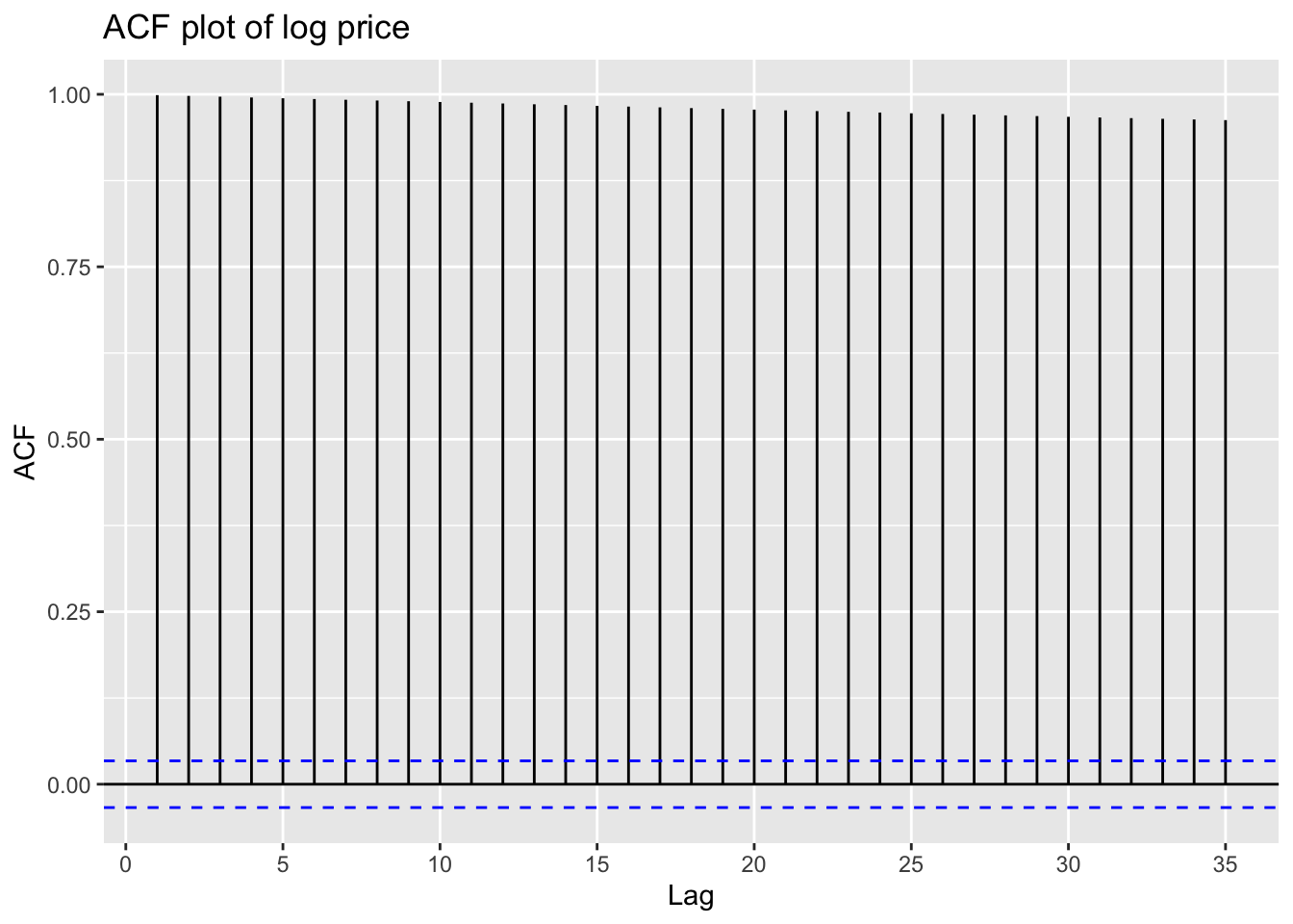

From this plot, it is evident that a differencing must be applied to this stock price data.

Code

ggAcf(returns)+ggtitle("ACF plot of log price with differencing")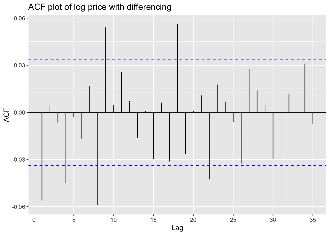

Code

ggPacf(returns)+ggtitle("PACF plot of log price with differencing")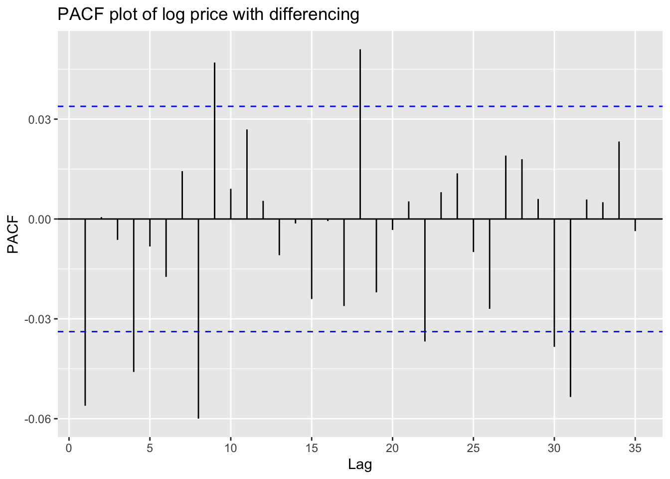

Code

ggAcf(abs(returns))+ggtitle("ACF plot of absolute log price with differencing")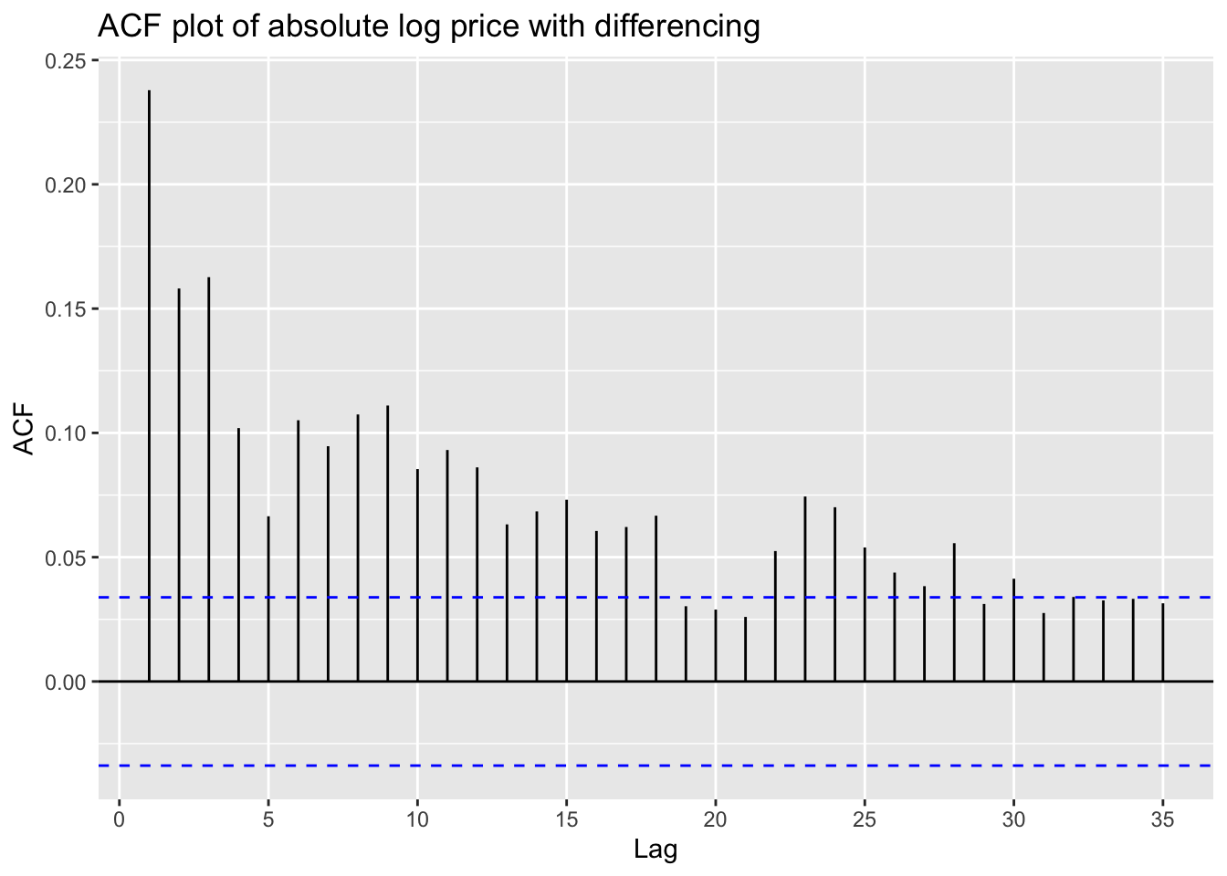

Code

ggAcf(returns^2)+ggtitle("ACF plot of squared log price with differencing")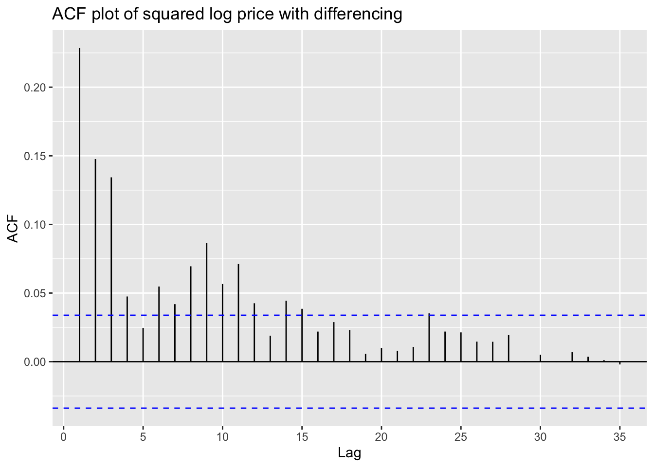

These plots above shows that an ARIMA model is needed for fitting this stock price data.

3 ARIMA model fitting

Next, I will try to fit a series of ARIMA models with different parameters and determine the best model based on AIC, BIC and AICc values.

Code

log.WMT=log(WMT.close)
i=1
temp= data.frame()
ls=matrix(rep(NA,6*18),nrow=18) 


for (p in 0:2)
{
  for(q in 0:2)
  {
    for(d in 0:1)
    {
      
      if(p+d+q<=8)
      {
        
        model<- Arima(log.WMT,order=c(p,d,q),include.drift=TRUE) 
        ls[i,]= c(p,d,q,model$aic,model$bic,model$aicc)
        i=i+1
      }
    }
  }
}

temp= as.data.frame(ls)
names(temp)= c("p","d","q","AIC","BIC","AICc")

#temp
knitr::kable(temp)

p	d	q	AIC	BIC	AICc
0	0	0	-4787.751	-4769.397	-4787.744
0	1	0	-20009.436	-19997.201	-20009.433
0	0	1	-8966.713	-8942.241	-8966.701
0	1	1	-20017.978	-19999.625	-20017.971
0	0	2	-11889.597	-11859.008	-11889.579
0	1	2	-20016.002	-19991.532	-20015.990
1	0	0	-20016.607	-19992.135	-20016.595
1	1	0	-20018.012	-19999.659	-20018.005
1	0	1	-20024.177	-19993.587	-20024.159
1	1	1	-20016.000	-19991.530	-20015.988
1	0	2	-20022.267	-19985.560	-20022.242
1	1	2	-20014.008	-19983.420	-20013.990
2	0	0	-20024.252	-19993.663	-20024.234
2	1	0	-20016.013	-19991.543	-20016.001
2	0	1	-20022.280	-19985.572	-20022.254
2	1	1	-20014.013	-19983.425	-20013.995
2	0	2	-20020.204	-19977.378	-20020.170
2	1	2	-20014.629	-19977.923	-20014.604

Model with minimum AIC:

Code

temp[which.min(temp$AIC),]

   p d q       AIC       BIC      AICc
13 2 0 0 -20024.25 -19993.66 -20024.23

Model with minimum BIC:

Code

temp[which.min(temp$BIC),]

  p d q       AIC       BIC      AICc
8 1 1 0 -20018.01 -19999.66 -20018.01

Model with minimum AICc:

Code

temp[which.min(temp$AICc),]

   p d q       AIC       BIC      AICc
13 2 0 0 -20024.25 -19993.66 -20024.23

The results shows that ARIMA(2,0,0) has minimum AIC and AICc values, while ARIMA(1,1,0) has the minimum BIC value. Now compare the two models using model diagnostics.

1. ARIMA(1,1,0) model:

Code

sarima(log.WMT,1,1,0)

initial  value -4.403305 
iter   2 value -4.404882
iter   2 value -4.404882
iter   2 value -4.404882
final  value -4.404882 
converged
initial  value -4.404923 
iter   1 value -4.404923
final  value -4.404923 
converged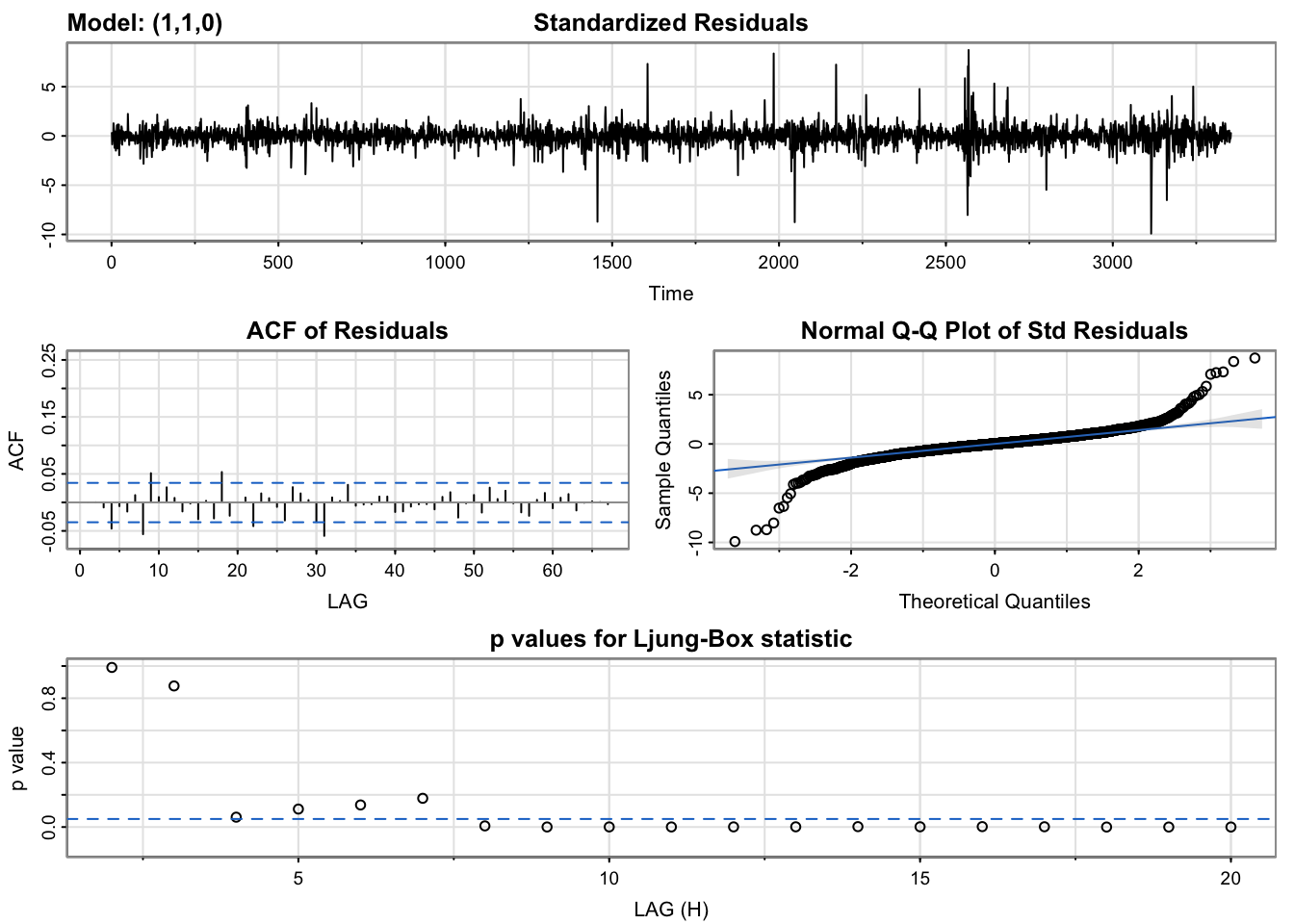

$fit

Call:
arima(x = xdata, order = c(p, d, q), seasonal = list(order = c(P, D, Q), period = S), 
    xreg = constant, transform.pars = trans, fixed = fixed, optim.control = list(trace = trc, 
        REPORT = 1, reltol = tol))

Coefficients:
          ar1  constant
      -0.0561     4e-04
s.e.   0.0172     2e-04

sigma^2 estimated as 0.0001493:  log likelihood = 10012.01,  aic = -20018.01

$degrees_of_freedom
[1] 3351

$ttable
         Estimate     SE t.value p.value
ar1       -0.0561 0.0172 -3.2545  0.0011
constant   0.0004 0.0002  1.9768  0.0481

$AIC
[1] -5.97018

$AICc
[1] -5.970179

$BIC
[1] -5.964706

2. ARIMA(2,0,0) model:

Code

sarima(log.WMT,2,0,0)

initial  value -0.871503 
iter   2 value -0.872504
iter   3 value -4.313351
iter   4 value -4.313868
iter   5 value -4.376908
iter   6 value -4.401093
iter   7 value -4.404339
iter   8 value -4.404343
iter   8 value -4.404343
final  value -4.404343 
converged
initial  value -4.403196 
iter   1 value -4.403196
final  value -4.403196 
converged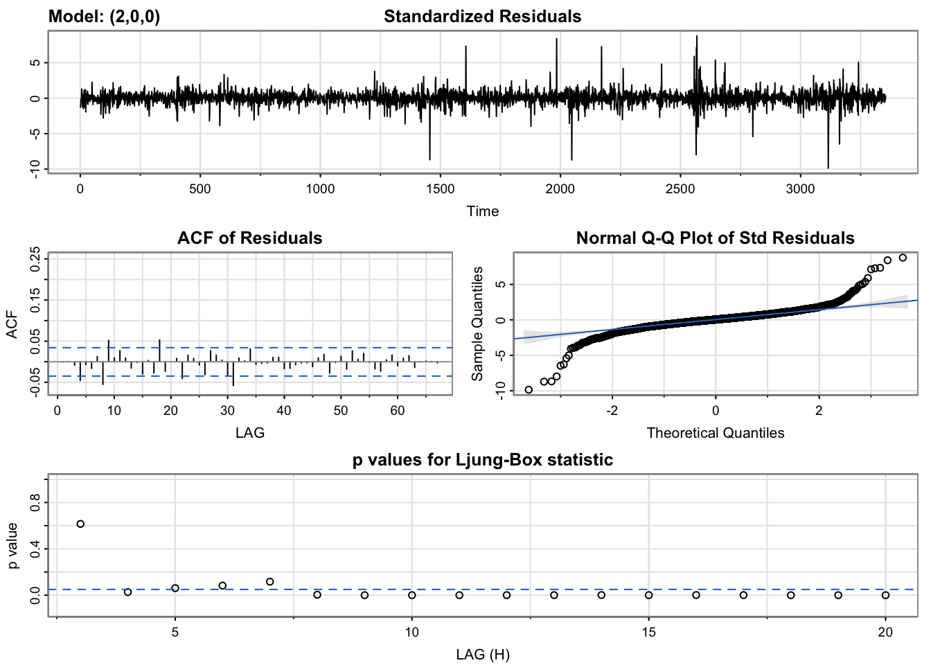

$fit

Call:
arima(x = xdata, order = c(p, d, q), seasonal = list(order = c(P, D, Q), period = S), 
    xreg = xmean, include.mean = FALSE, transform.pars = trans, fixed = fixed, 
    optim.control = list(trace = trc, REPORT = 1, reltol = tol))

Coefficients:
         ar1     ar2   xmean
      0.9449  0.0548  4.3072
s.e.  0.0172  0.0172  0.3959

sigma^2 estimated as 0.0001494:  log likelihood = 10009.2,  aic = -20010.4

$degrees_of_freedom
[1] 3351

$ttable
      Estimate     SE t.value p.value
ar1     0.9449 0.0172 54.7973  0.0000
ar2     0.0548 0.0172  3.1790  0.0015
xmean   4.3072 0.3959 10.8783  0.0000

$AIC
[1] -5.96613

$AICc
[1] -5.966128

$BIC
[1] -5.958834

According to model diagnostics of these two models, we can see that both models perform relatively good. The residuals of both models have good normality and coefficients in these two models are all significant. However, from the Ljung-Box test, ARIMA(1,1,0) has more values greater than 0.05, which means the residuals of this model are more likely to be independent. Thus, I will choose ARIMA(1,1,0) as the optimal model.

The squared residuals of this model is as follows:

Code

arima1=arima(log.WMT,order=c(1,1,0))

res.arima1=arima1$res
squared.res.arima1=res.arima1^2
plot(squared.res.arima1,main='Squared Residuals')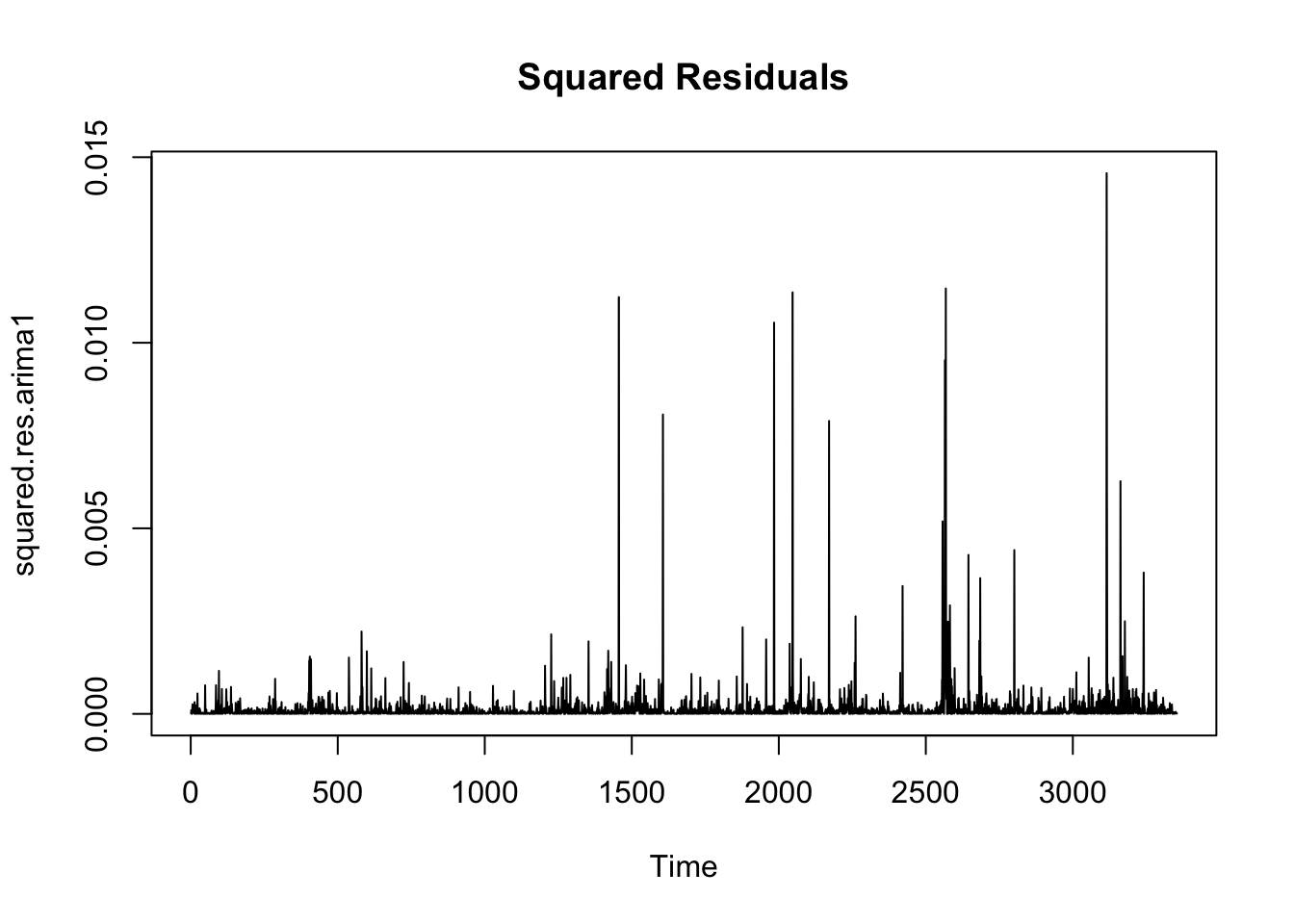

Obviously, an ARCH model is needed for fitting the residuals of ARIMA model.

4 ARCH model fitting

In following part, I will sequentially fit ARCH models with different parameters and determine the best one based on AIC value.

Code

ARCH <- list()
i=1
for (p in 1:10) {
ARCH[[i]] <- garch(res.arima1,order=c(0,p),trace=F)
i=i+1
} 

## get AIC values for model evaluation
ARCH_AIC <- sapply(ARCH, AIC) 

Minimum AIC value:

[1] -20477.34

The parameter of model with minimum AIC value:

[1] 8

This means ARCH(8) fits the residual best. Have a look at the summary of this model.

Code

arch8=garch(res.arima1,order=c(0,8),trace=F)
summary(arch8)

Call:
garch(x = res.arima1, order = c(0, 8), trace = F)

Model:
GARCH(0,8)

Residuals:
      Min        1Q    Median        3Q       Max 
-10.21902  -0.49084   0.05551   0.56775   9.64066 

Coefficient(s):
    Estimate  Std. Error  t value Pr(>|t|)    
a0 7.317e-05   2.101e-06   34.819  < 2e-16 ***
a1 1.187e-01   1.289e-02    9.212  < 2e-16 ***
a2 4.500e-02   1.274e-02    3.532 0.000413 ***
a3 6.045e-02   1.156e-02    5.230 1.70e-07 ***
a4 6.918e-02   1.453e-02    4.761 1.93e-06 ***
a5 1.663e-13   9.013e-03    0.000 1.000000    
a6 1.103e-02   1.050e-02    1.050 0.293590    
a7 1.060e-01   7.161e-03   14.802  < 2e-16 ***
a8 1.018e-01   1.172e-02    8.687  < 2e-16 ***
---
Signif. codes:  0 '***' 0.001 '**' 0.01 '*' 0.05 '.' 0.1 ' ' 1

Diagnostic Tests:
    Jarque Bera Test

data:  Residuals
X-squared = 25923, df = 2, p-value < 2.2e-16


    Box-Ljung test

data:  Squared.Residuals
X-squared = 0.0079708, df = 1, p-value = 0.9289

The p-value of Box-Ljung test is much greater than 0.05, suggesting that this model has adequately represents the residual. Also, most coefficients within this model are significant except a5 and a6.

5 Model diagnostics and conclusions

Finally, have a look at the model diagnostics of the whole ARIMA(1,1,0)+ARCH(8) for this stock price data to check the model performance.

Code

checkresiduals(arch8)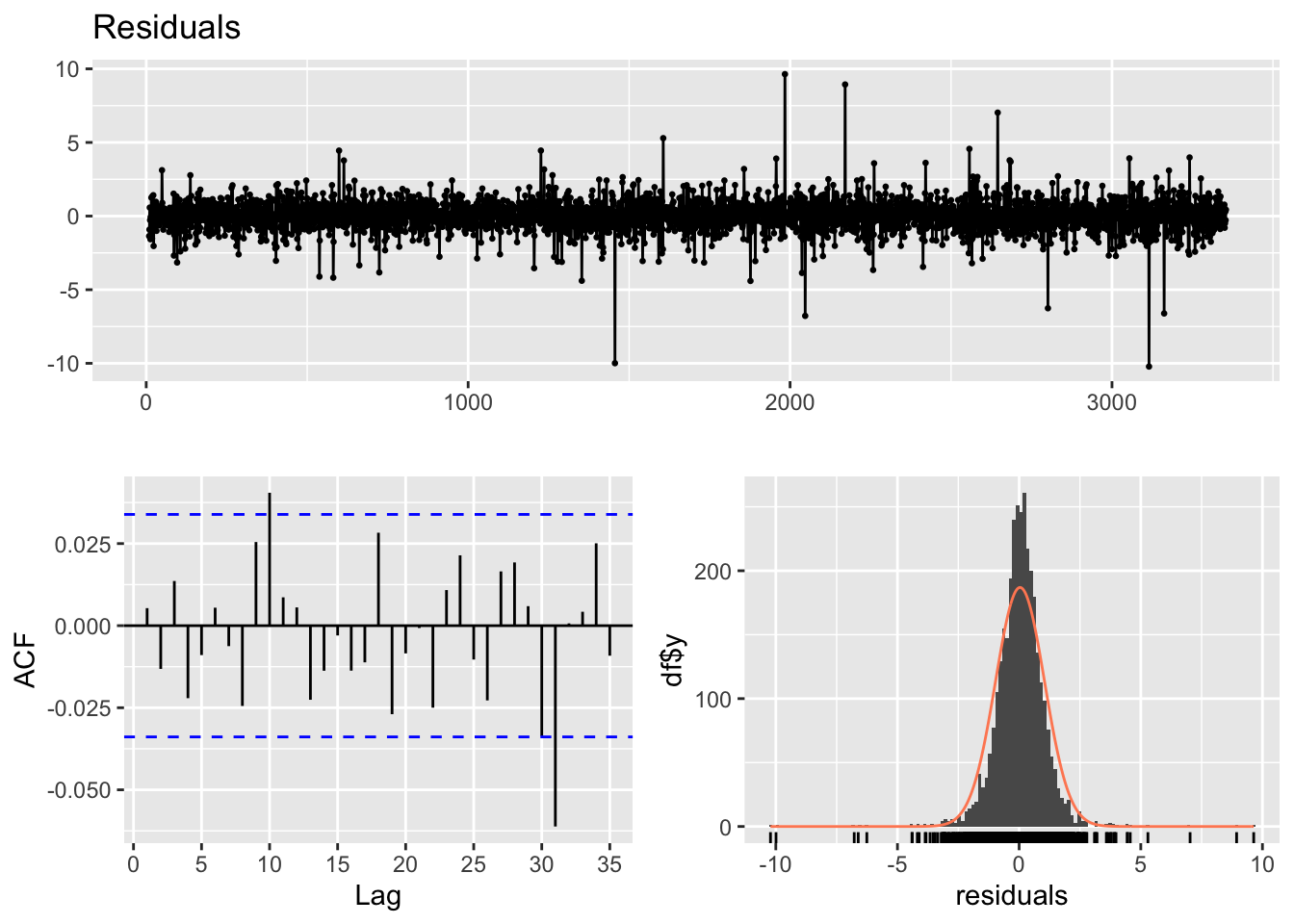

Code

qqnorm(arch8$residuals, pch=1)
qqline(arch8$residuals, col="red", lwd=2)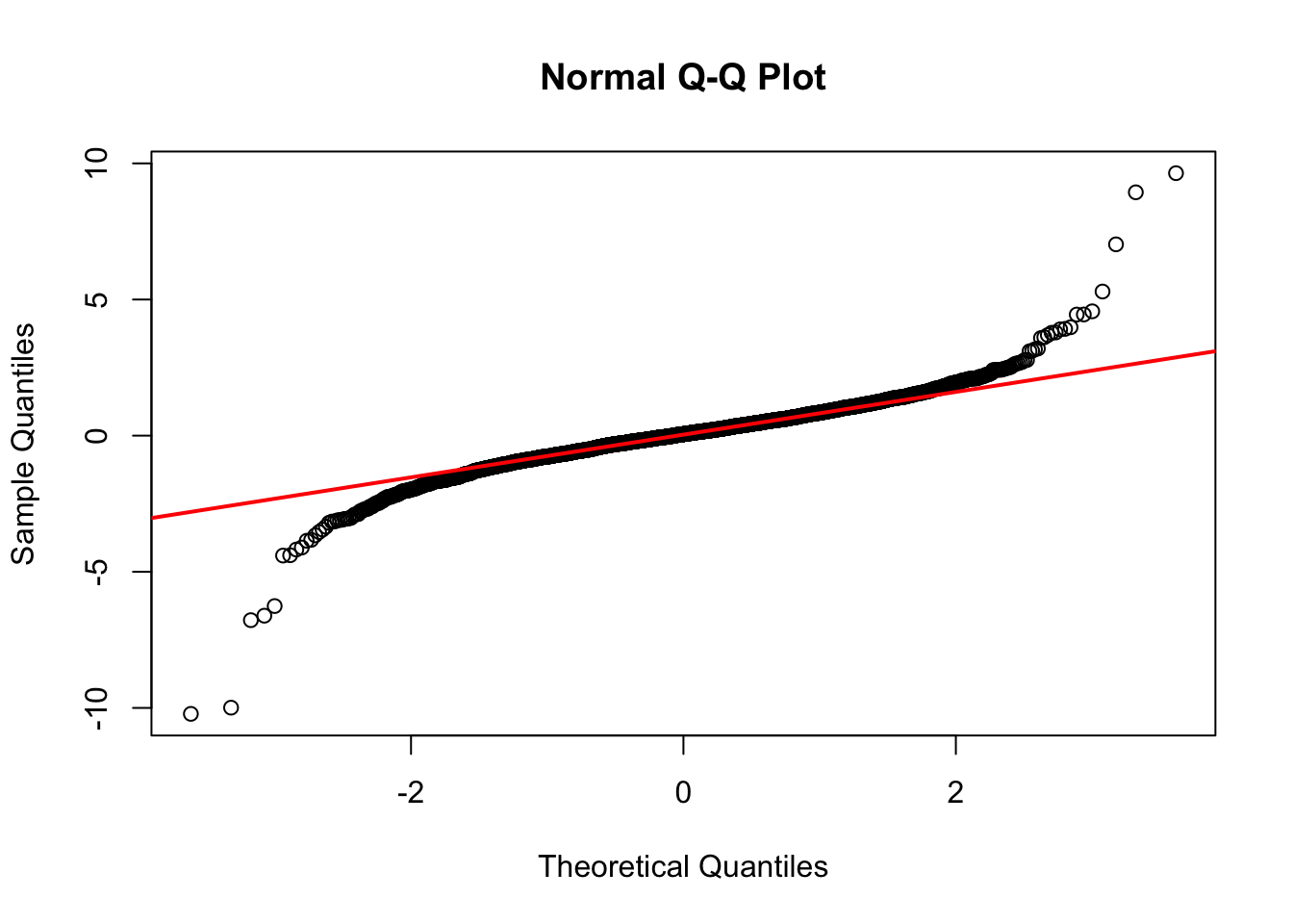

Code

Box.test(arch8$residuals, type="Ljung-Box")

    Box-Ljung test

data:  arch8$residuals
X-squared = 0.095367, df = 1, p-value = 0.7575

These plots and test all show strong signals that the model performs quite well. From the residual plot, we can see relatively constant mean and variance. Next, the ACF plot shows good stationarity within the residuals. Besides, the distribution of the residuals and QQ-plot indicate that the residuals almost follow a normal distribution. Finally, the p-value of Box-Ljung test is much greater than 0.05, meaning that the residuals are independent.

6 Model equations

The equations of the ARIMA(1,1,0)+ARCH(8) model can be written as follows:

\[ (1-\phi_1B)(1-B)x_t=y_t+\delta \]

\[ y_t=\sigma_t \epsilon_t \]

\[ \sigma^2=a_0+a_1y_{t-1}^2+a_2y_{t-2}^2+a_3y_{t-3}^2+\cdots+a_8y_{t-8}^2 \]

In these equations, \(\phi_1\) eqauls to -0.0561. The coefficients of the third equations are listed below:

[[1]]

Call:
garch(x = res.arima1, order = c(0, p), trace = F)

Coefficient(s):
       a0         a1         a2         a3         a4         a5         a6  
7.317e-05  1.187e-01  4.500e-02  6.045e-02  6.918e-02  1.663e-13  1.103e-02  
       a7         a8  
1.060e-01  1.018e-01  

7 Stock price and sales

In this section, I will compare the visualizations of stock price and weekly sales, in order to figure out if these two time series have something in common. The observation time is from 2010-02 to 2012-10.

[1] "WMT"

Code

chartSeries(WMT, theme = chartTheme("white"),
            bar.type = "hlc",
            up.col = "green", 
            dn.col = "red")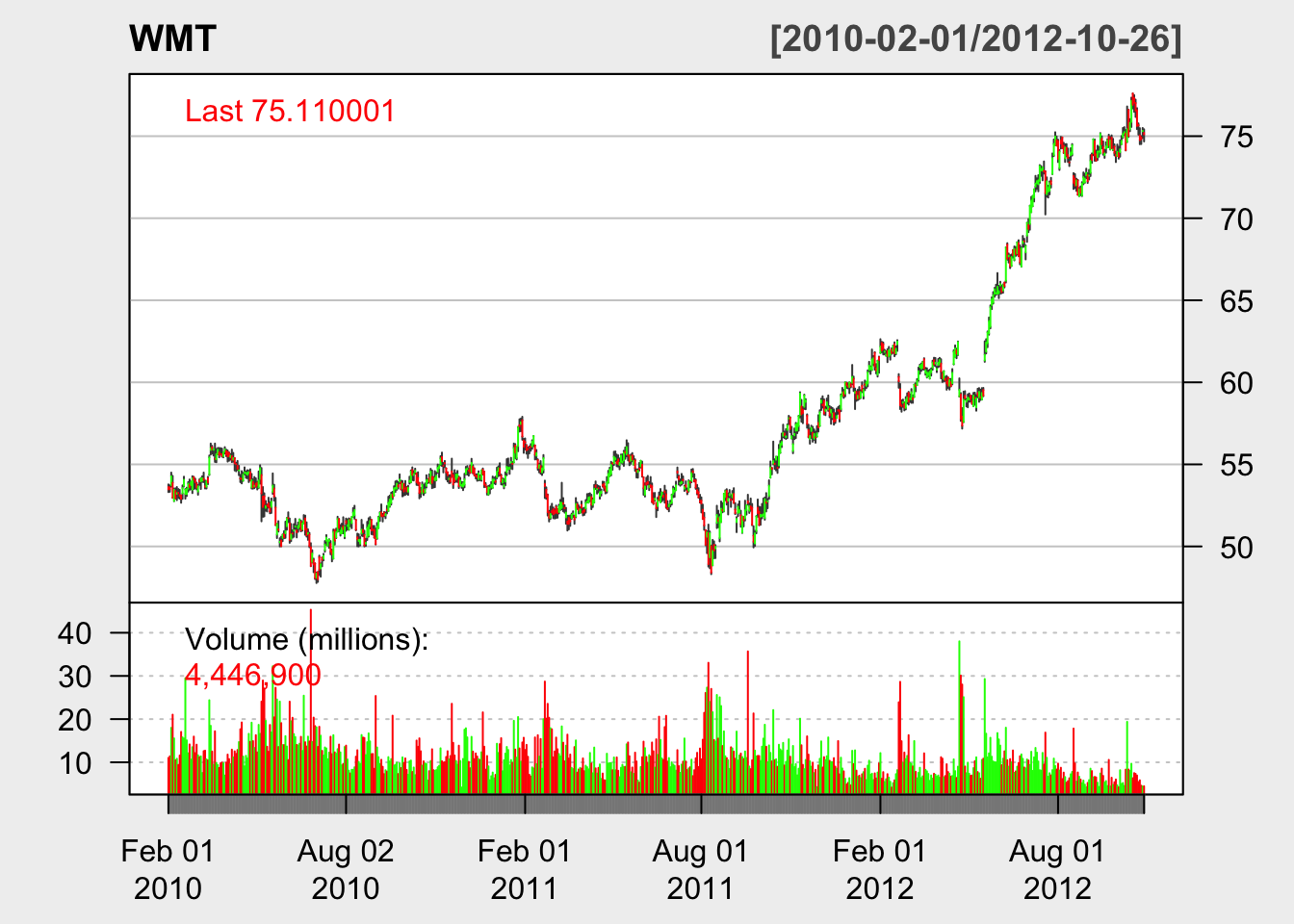

Code

gglagplot(WMT.close, do.lines=FALSE, lags=1)+xlab("Lag 1")+ylab("Yi")+ggtitle("Lag Plot for Stock Price")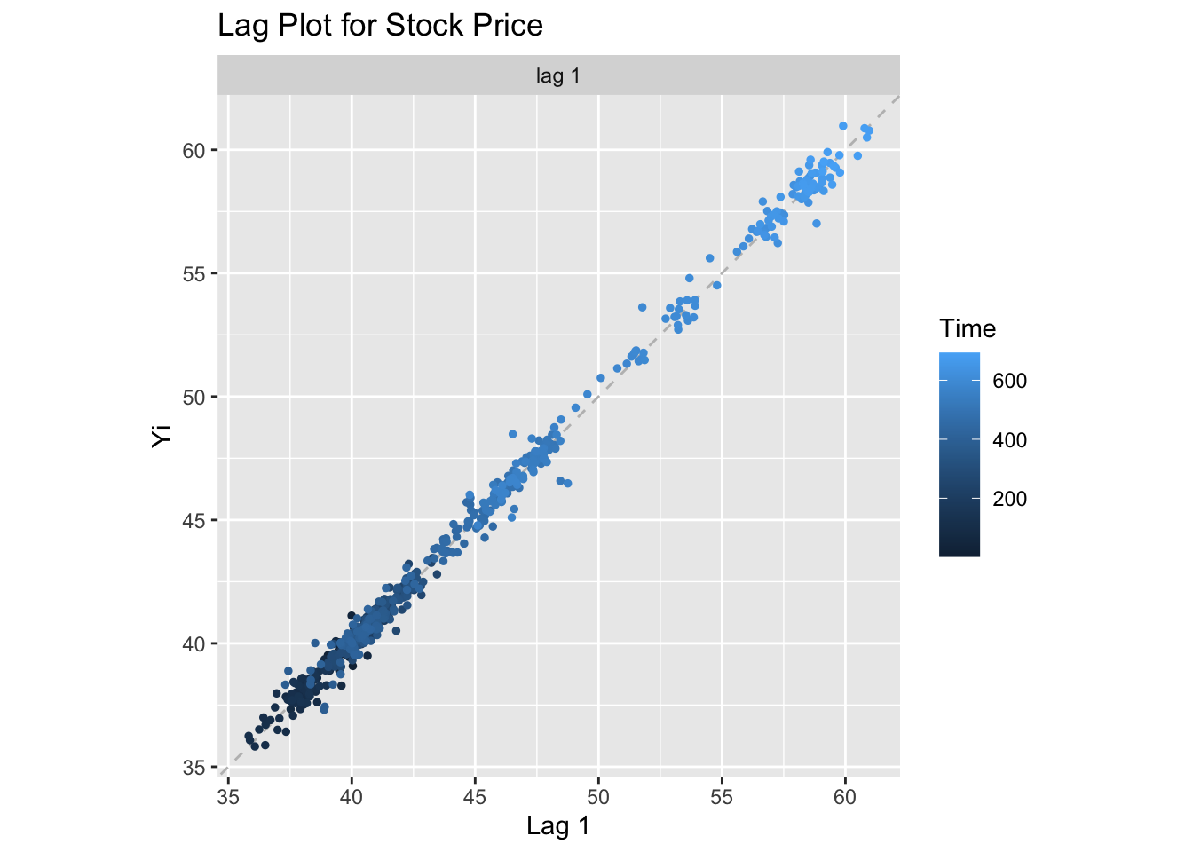

The candlestick plot and lag plot indicate that the stock price of Walmart from 2010 to 2012 has a obvious upward trend. However, the “decompose” function failed to decompose this time series into different components, suggesting that seasonality does not exist in this time series.

Code

walmart=read.csv("./data/Walmart_sales_data.csv")

bytime=group_by(walmart,Date)
sales=summarise(bytime,avg = mean(Weekly_Sales))
sales$Date=as.Date(sales$Date)


ggplot(sales,aes(x=Date,y=avg))+
  geom_line()+
  labs(
    x = "Time",
    y = "Weekly sales"
  )+
  ggtitle("Average Weekly sales from 2010 to 2012")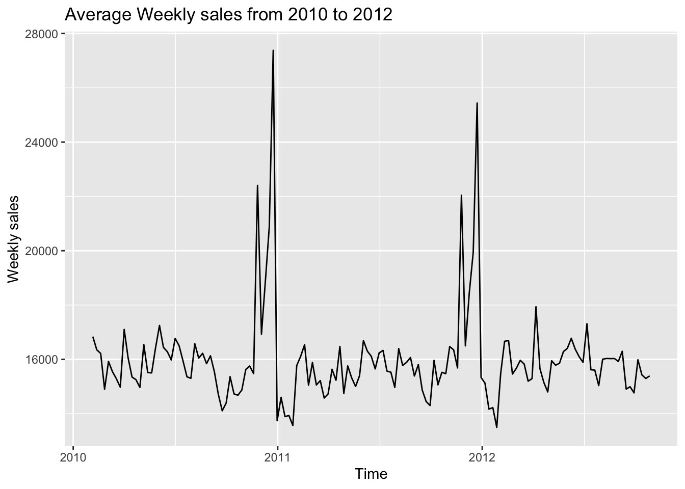

This plot above, which we are already very familiar, displays the average weekly sales of all the stores from 2010 to 2012. This time series of weekly sales has significant seasonal components rather than trend, which is absolutely opposite to the stock price data. Therefore, we can not observe any relationship between the stock price of Walmart and the weekly sales of given stores.