ARIMAX/SARIMAX Models

1 Literature review

Sales forecasting is crucial for companies to plan their operations and make informed decisions about future sales goals. According to some cases of sales forecasting on the internet, the variables that are important for the forecasting can vary by the industry, business type and specific product. However, there are still many common factors which are essential for most sales forecasting.

There are mainly two types of factors that need to be consider during forecasting: external factors and internal factors. The former ones include population, market environment and economic situation, while the latter ones mainly contain the company’s historical sales data, marketing and advertising strategies, and product lifecycle.

For this project that focuses on sales forecasting for Walmart data, I will consider several features that may contribute to the forecasting of the sales data. First of all, fuel price and local unemployment rate should be taken into consideration, because they are indirectly or directly related to the economic environment. Secondly, the CPI index is also important since it highly relates to the consumers and reflects the level of inflation. Besides, since many products have seasonal effects and can be related to the temperature, I will also include temperature as one of the predictor variables.

2 Variables and visualization

In this project, weekly sales is the response variable, while fuel price, temperature, CPI index and unemployment rate are predictor variables.

First, have a quick look of the data table after merging and cleaning which is ready for model fitting.

Code

walmart=read.csv("./data/Walmart_sales_data.csv")
type=read.csv("./data/Walmart_stores.csv")
features=read.csv("./data/Walmart_features.csv")

df=merge(walmart,type,by="Store")
df_all=merge(df, features, by=c("Date","Store"))

A_bytime=group_by(df_all[df_all$Type=='A',],Date)
A_sales=summarise(A_bytime,sales = mean(Weekly_Sales),fuel_price=mean(Fuel_Price),
                  temperature=mean(Temperature),CPI=mean(CPI),unemployment=mean(Unemployment))

B_bytime=group_by(df_all[df_all$Type=='B',],Date)
B_sales=summarise(B_bytime,sales = mean(Weekly_Sales),fuel_price=mean(Fuel_Price),
                  temperature=mean(Temperature),CPI=mean(CPI),unemployment=mean(Unemployment))

C_bytime=group_by(df_all[df_all$Type=='C',],Date)
C_sales=summarise(C_bytime,sales = mean(Weekly_Sales),fuel_price=mean(Fuel_Price),
                  temperature=mean(Temperature),CPI=mean(CPI),unemployment=mean(Unemployment))

knitr::kable(
  head(A_sales)
)

Date	sales	fuel_price	temperature	CPI	unemployment
2010-02-05	21259.34	2.702128	34.04677	170.5586	8.443993
2010-02-12	20491.12	2.683142	33.28542	170.4538	8.439380
2010-02-19	20408.21	2.656316	36.61275	170.4040	8.446582
2010-02-26	18598.27	2.675451	38.86468	170.7273	8.432503
2010-03-05	19881.15	2.721852	42.38552	170.8344	8.438802
2010-03-12	19532.97	2.761870	47.78439	170.8610	8.436977

Code

df=A_sales[,2:6]
temp.ts=ts(df, start=decimal_date(as.Date("2010-02-05")), frequency = 365.25/7)
autoplot(temp.ts,facets=TRUE)+
  xlab("Year")+
  ylab("Value")+
  ggtitle("Weekly sales and 4 predictor variables")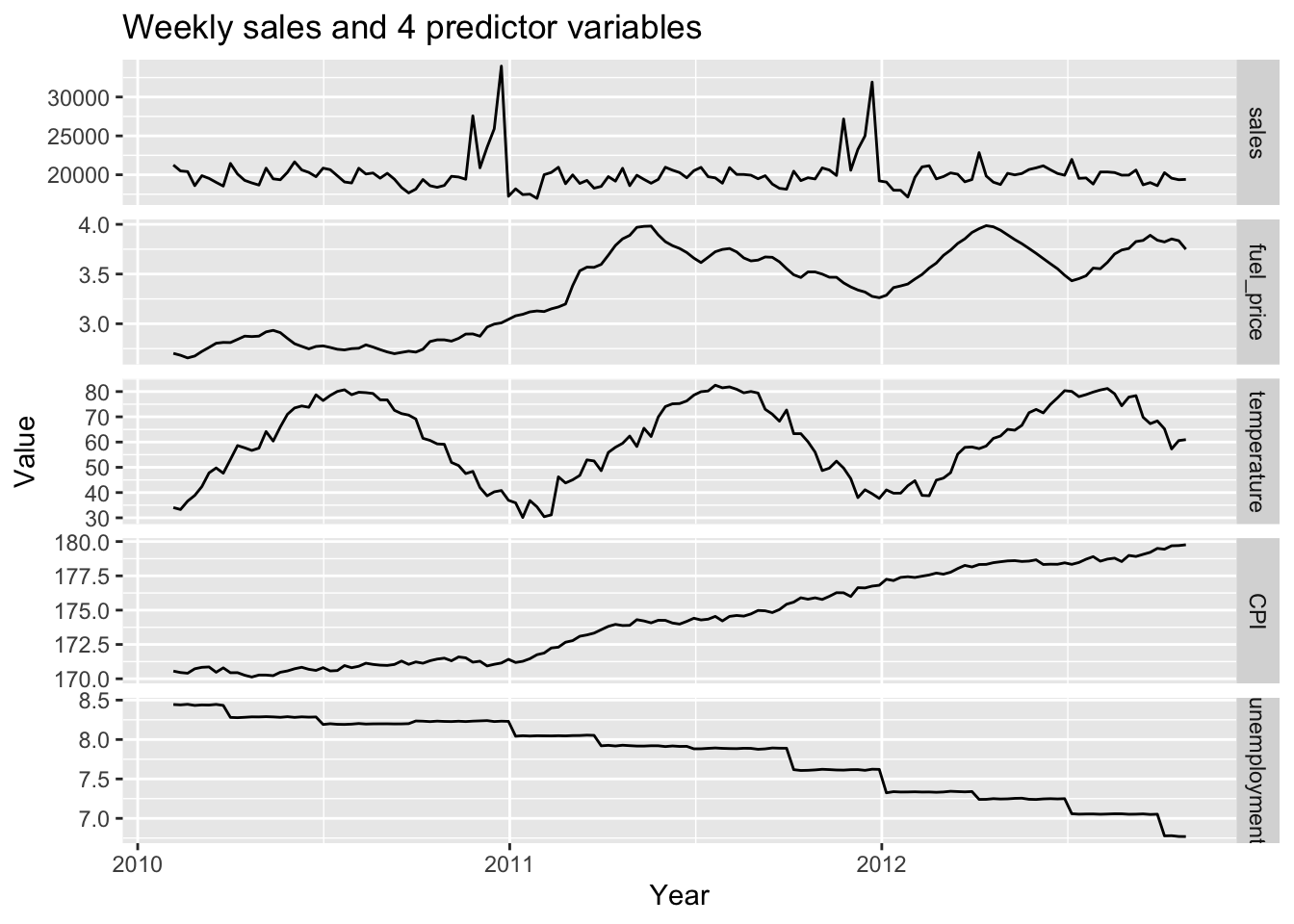

This is a visualization of weekly sales and other variables from 2010 to 2012. It is noticed that most variables have different trends within the observation time.

3 Auto.arima fitting

Code

xreg <- cbind(fuel = temp.ts[, "fuel_price"],
              tem = temp.ts[, "temperature"],
              cpi = temp.ts[, "CPI"],
              unemp = temp.ts[, "unemployment"])

fit <- auto.arima(temp.ts[, "sales"], xreg = xreg)
summary(fit)

Series: temp.ts[, "sales"] 
Regression with ARIMA(0,0,0)(0,1,0)[52] errors 

Coefficients:
           fuel      tem       cpi      unemp
      -251.0014  45.0867   20.4911  -292.1289
s.e.   223.2053  22.3984  104.5482   623.5498

sigma^2 = 621301:  log likelihood = -733.92
AIC=1477.84   AICc=1478.55   BIC=1490.4

Training set error measures:
                    ME     RMSE      MAE         MPE    MAPE      MASE
Training set -2.770906 614.1811 345.2601 -0.00187349 1.69265 0.5876295
                  ACF1
Training set 0.1379488

Code

checkresiduals(fit)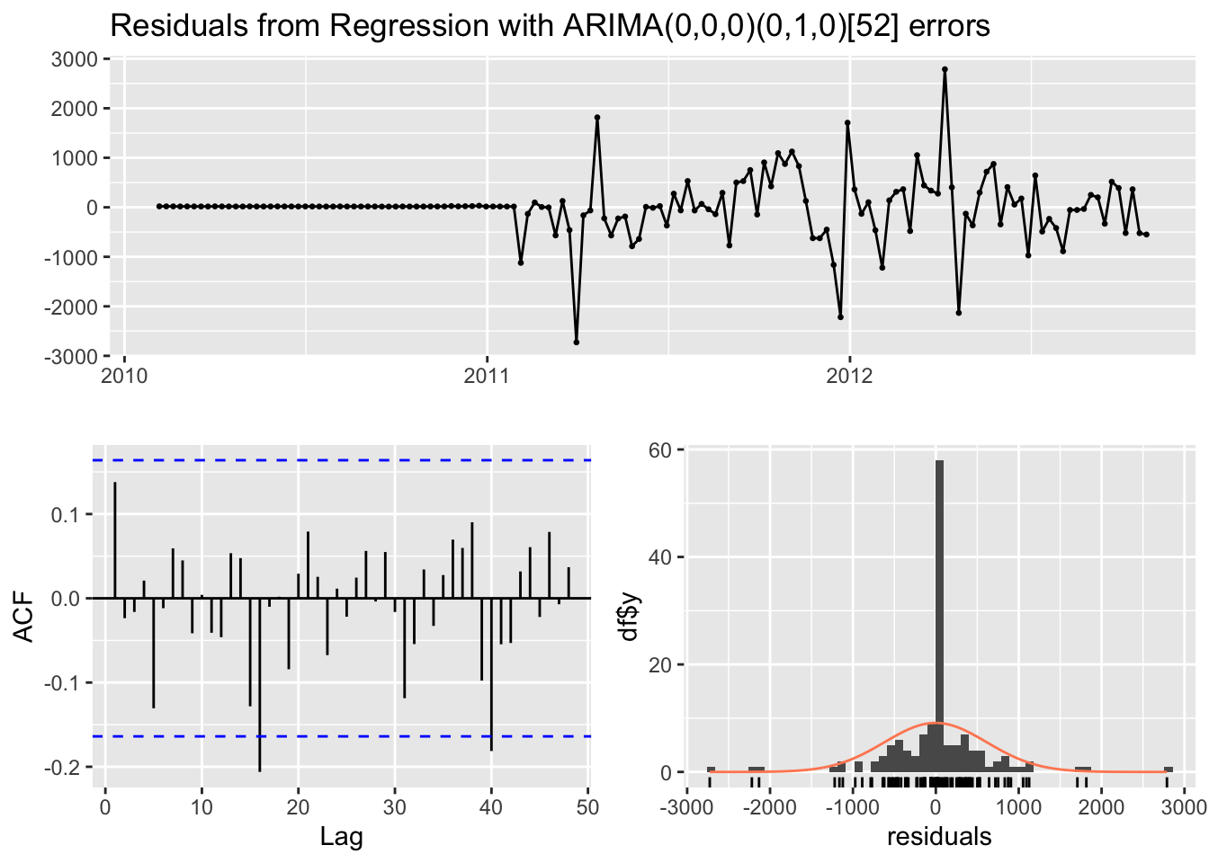

    Ljung-Box test

data:  Residuals from Regression with ARIMA(0,0,0)(0,1,0)[52] errors
Q* = 22.321, df = 29, p-value = 0.8067

Model df: 0.   Total lags used: 29

As we can see, the auto.arima() function fits a regression with SARIMA(0,0,0)(0,1,0)[52] errors, which is a SARIMAX model. The Ljung-Box test indicates that the residuals are independent and the model fits the data well.

4 Manually fitting

First, fit the linear regression model predicting weekly sales using 4 predictor variables.

Code

fit.reg=lm(sales~. , data=df)
summary(fit.reg)

Call:
lm(formula = sales ~ ., data = df)

Residuals:
    Min      1Q  Median      3Q     Max 
-3563.8 -1030.1  -153.0   440.2 13763.0 

Coefficients:
               Estimate Std. Error t value Pr(>|t|)  
(Intercept)  -114645.61   71035.82  -1.614   0.1088  
fuel_price     -1353.55     807.54  -1.676   0.0960 .
temperature      -14.40      12.33  -1.168   0.2447  
CPI              651.76     330.64   1.971   0.0507 .
unemployment    3396.72    1968.00   1.726   0.0866 .
---
Signif. codes:  0 '***' 0.001 '**' 0.01 '*' 0.05 '.' 0.1 ' ' 1

Residual standard error: 2170 on 138 degrees of freedom
Multiple R-squared:  0.04536,   Adjusted R-squared:  0.01769 
F-statistic: 1.639 on 4 and 138 DF,  p-value: 0.1679

From the p-value, we can find that temperature is not significant at all, while other three predictor variables are significant under 0.1 level.

Let’s have a look at the residuals:

Code

res.fit=ts(residuals(fit.reg), start=decimal_date(as.Date("2010-02-05")), frequency = 365.25/7)
autoplot(res.fit)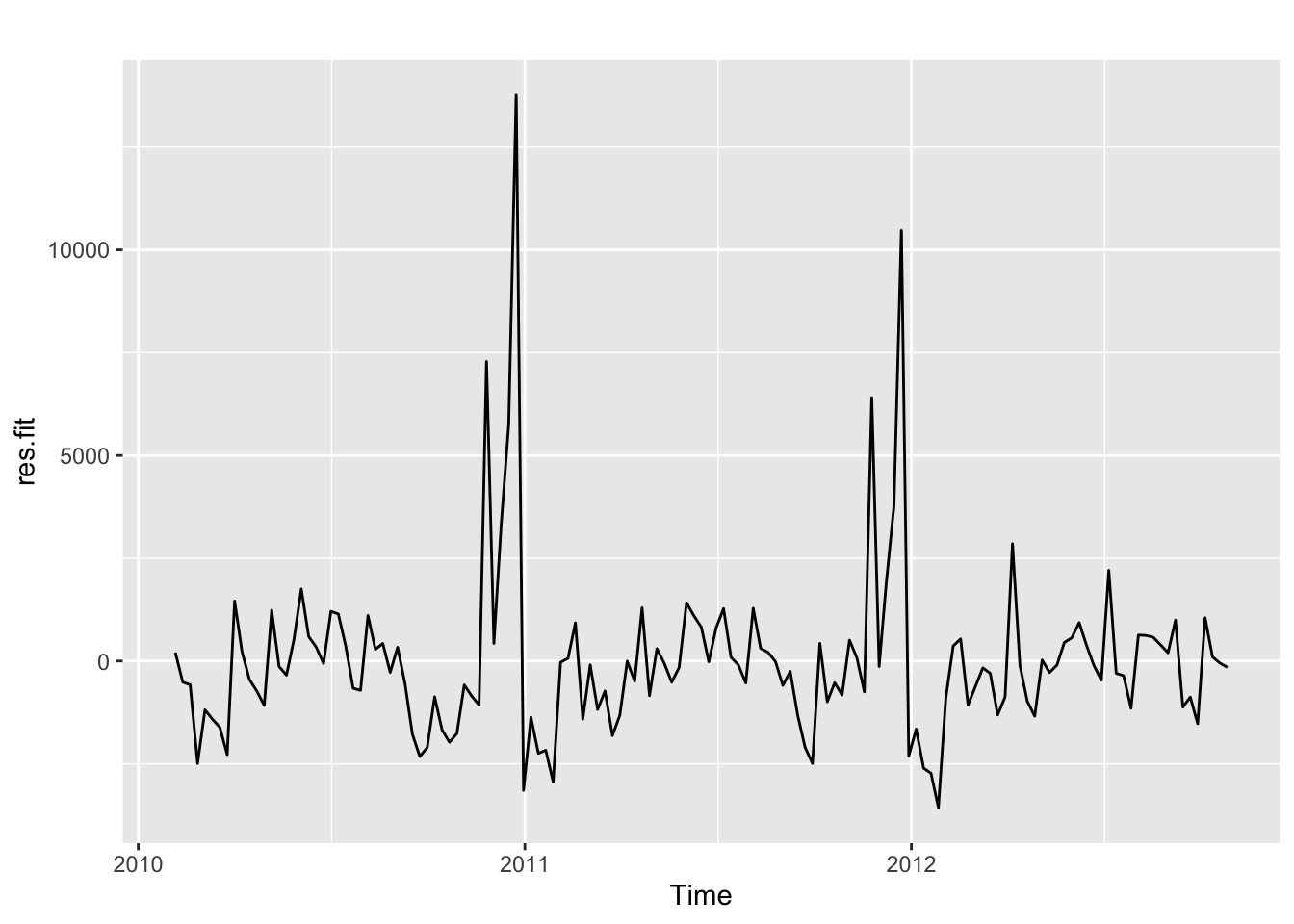

Differencing with lag=52:

Code

res.fit %>% diff(52) %>% ggtsdisplay()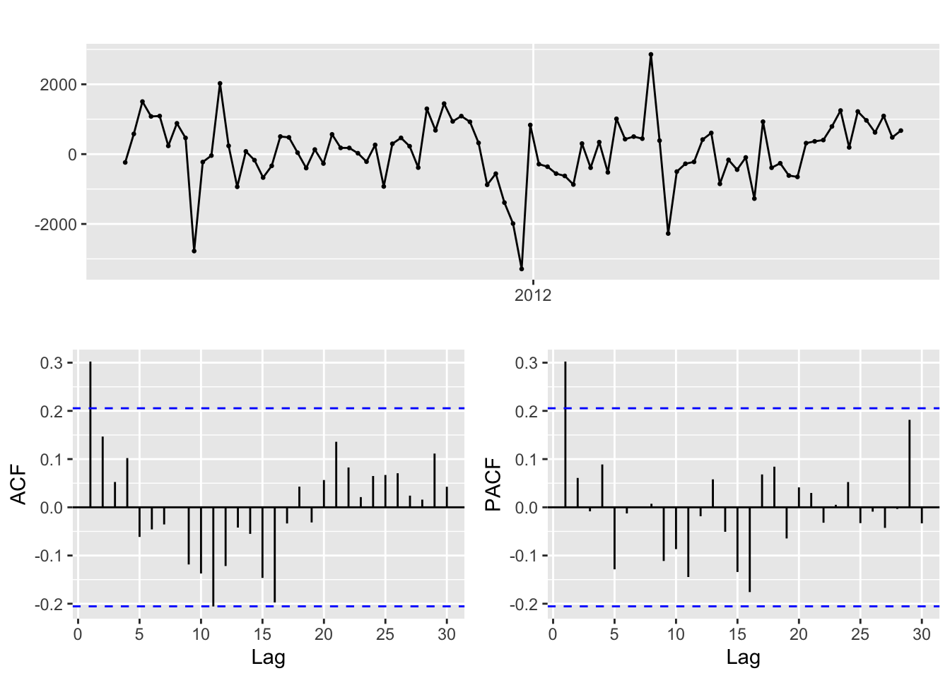

There seems to exist seasonal component in the residuals. When applying a lag 52 differencing to the residuals, it becomes quite stationary. Use SARIMA model to fit the residuals now.

Code

i=1
ls=matrix(rep(NA,9*30),nrow=30) 

for (p in 0:1)
{
  for(q in 0:1)
  {
    for(P in 0:1)
    {
      for(Q in 0:1)
        {
        for(d in 0:1){
          model<- try(Arima(res.fit,order=c(p,d,q),seasonal=c(P,1,Q)),silent = TRUE)
          if('try-error' %in% class(model)){
            next
            }else{
            ls[i,]= c(p,d,q,P,1,Q,model$aic,model$bic,model$aicc)
            i=i+1
          }
        }
      }
    }
  }
}

temp= as.data.frame(ls)
names(temp)= c("p","d","q","P","D","Q","AIC","BIC","AICc")

   p d q P D Q      AIC      BIC     AICc
26 1 1 1 0 1 0 1486.177 1493.676 1486.456

The SARIMA(1,1,1,0,1,0)[52] has fitted the residuals best and have minimum AIC, BIC and AICc.

Code

fit=Arima(res.fit,order=c(1,1,1),seasonal=c(0,1,0))
summary(fit) 

Series: res.fit 
ARIMA(1,1,1)(0,1,0)[52] 

Coefficients:
         ar1      ma1
      0.3149  -1.0000
s.e.  0.1011   0.0389

sigma^2 = 796548:  log likelihood = -740.09
AIC=1486.18   AICc=1486.46   BIC=1493.68

Training set error measures:
                    ME     RMSE      MAE       MPE     MAPE      MASE
Training set -16.61097 700.1311 401.0234 -124.8012 248.4826 0.5792466
                    ACF1
Training set -0.02621394

Code

checkresiduals(fit)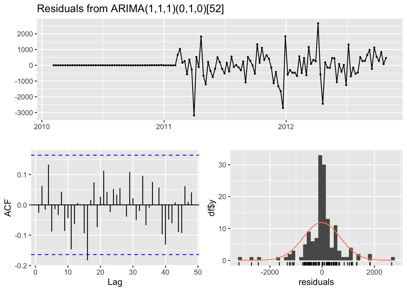

    Ljung-Box test

data:  Residuals from ARIMA(1,1,1)(0,1,0)[52]
Q* = 25.465, df = 27, p-value = 0.5484

Model df: 2.   Total lags used: 29

The model diagnostics above also indicates that this SARIMAX model fits the residuals well.

5 Cross-validation

In this part, I will use cross-validation to compare the RMSE of manually selected model and the model chosen by auto.arima. In practice, k equals to 100, and I predict the weekly sales of the next whole month in each iteration.

Code

n=length(res.fit)
k=100
freq=365.25/7
st=tsp(res.fit)[1]+k/freq

rmse1=matrix(NA, 10, 1)
rmse2=matrix(NA, 10, 1)

for (i in 1:10){
  xtrain=window(res.fit, end=st+(i-1)*4/freq)
  xtest=window(res.fit, start=st+(i-1)*4/freq+1/freq, end=st+i*4/freq)
  
  fit1 <- Arima(xtrain, order=c(1,1,1), seasonal=list(order=c(0,1,0), period=52),
                 method="ML")
  fcast1 <- forecast(fit1, h=4)
  fit2 <- Arima(xtrain, order=c(0,0,0), seasonal=list(order=c(0,1,0), period=52),
                 method="ML")
  fcast2 <- forecast(fit2, h=4)
  
  rmse1[i,1] <- sqrt(mean((fcast1$mean-xtest)^2))
  rmse2[i,1] <- sqrt(mean((fcast2$mean-xtest)^2))
}

plot(rmse1, type="l", col=2, xlab="horizon", ylab="RMSE")
lines(rmse2, type="l",col=3)
legend("topleft",legend=c("Manual","Auto"),col=2:4,lty=1)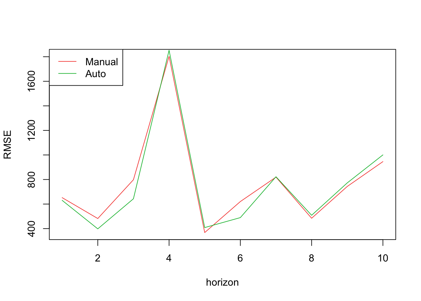

According to this plot, RMSE on test sets are very close for these two models. In these 10 iterations, the manually selected model beats the other one for 6 times, suggesting that this manually selected SARIMAX model performs slightly better.

Code

fit=Arima(temp.ts[, "sales"], order=c(1,1,1), seasonal=c(0,1,0), xreg = xreg)
summary(fit)

Series: temp.ts[, "sales"] 
Regression with ARIMA(1,1,1)(0,1,0)[52] errors 

Coefficients:
         ar1      ma1      fuel      tem       cpi      unemp
      0.1542  -0.9999  237.1454  42.1104   54.6488  -1327.677
s.e.  0.1084   0.0379  434.8001  22.5373  123.4687   1010.681

sigma^2 = 616978:  log likelihood = -726.64
AIC=1467.29   AICc=1468.65   BIC=1484.79

Training set error measures:
                   ME     RMSE      MAE       MPE     MAPE      MASE       ACF1
Training set 36.18888 602.0138 341.3975 0.1889309 1.673946 0.5810554 0.00182261

Therefore, the final model we choose is the SARIMAX model combined with a regression of 4 predictor variables, fuel price, temperature, CPI index and unemployment rate, and a SARIMA(1,1,1,0,1,0)[52] model fitting the residuals.

6 Forecasting

First use auto.arima() function to fit and forecast 4 predictor variables and then forecast the response variable weekly sales.

Code

fuel_fit<-auto.arima(df$fuel_price)
temp_fit<-auto.arima(df$temperature)
cpi_fit<-auto.arima(df$CPI)
unemp_fit<-auto.arima(df$unemployment)

fuel_f<-forecast(fuel_fit)
temp_f<-forecast(temp_fit)
cpi_f<-forecast(cpi_fit)
unemp_f<-forecast(unemp_fit)

fxreg <- cbind(fuel = fuel_f$mean,
               tem = temp_f$mean,
               cpi = cpi_f$mean,
               unemp = unemp_f$mean)

fcast <- forecast(fit, xreg=fxreg) 
autoplot(fcast) + xlab("Time") +
  ylab("Weekly Sales")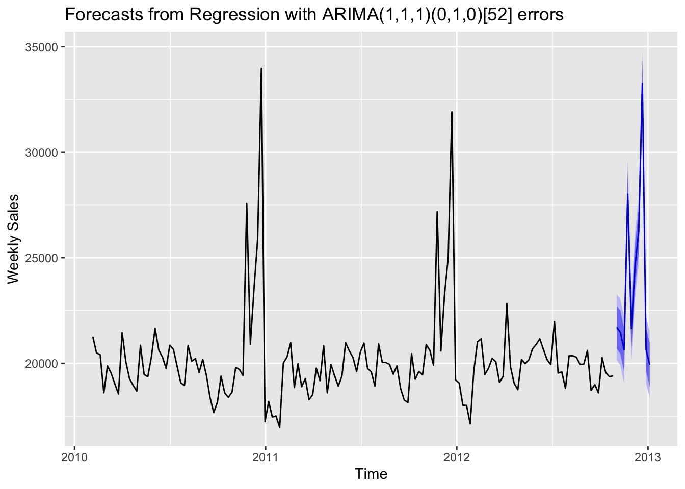

This forecasting shows that the SARIMAX model has effectively captured the data pattern, especially the seasonality in this data, and generated relatively good results based on 4 predictor variables. Rather than only using historical sales data to construct a SARIMA time series model, SARIMAX can deal with the sales data more comprehensively since it also takes CPI index, unemployment rate and fuel price into consideration.